As deep learning continues its meteoric rise in computer vision and multimodal sensing, deploying high‑performance models on resource‑constrained edge devices remains a major hurdle. Enter Layered Self‑Supervised Knowledge Distillation (LSSKD)—an innovative framework that leverages self‑distillation across multiple network stages to produce compact, high‑accuracy student models without relying on massive pre‑trained teachers.
In this article, we’ll explore 7 incredible upsides and downsides of LSSKD for edge computing, covering:
- What LSSKD is and why it matters
- Key advantages that make LSSKD a game‑changer
- Potential limitations to watch out for
- Best practices for implementation
- Real‑world use cases
- SEO keywords woven naturally for discoverability
- A strong call‑to‑action to get you started
Whether you’re an AI engineer, product manager, or tech journalist, this guide will equip you with the insights needed to decide if LSSKD belongs in your next edge AI project.
1. What Is Layered Self‑Supervised Knowledge Distillation?
Knowledge Distillation has long been used to compress large “teacher” networks into smaller “student” models by transferring soft‑label information. Traditional methods focus only on the final outputs, ignoring the wealth of hierarchical knowledge in intermediate layers.
LSSKD changes the game by:
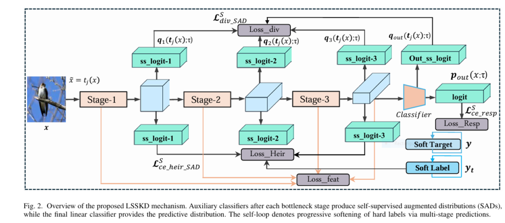
- Adding auxiliary classifiers after each bottleneck stage in the student network.
- Generating Self‑Supervised Augmented Distributions (SADs) via transformations (e.g., rotations) to soften labels at multiple levels.
- Employing cross‑layer KL divergence and L₂ feature alignment losses to enforce consistency.
- Removing all auxiliary branches at inference, so there’s zero extra compute cost on edge devices.
By harnessing hierarchical label softening and cross‑layer distillation, LSSKD achieves state‑of‑the‑art performance on CIFAR‑100 and ImageNet, while keeping the student model lightweight and efficient .
2. Upside #1: Superior Accuracy on Tiny Models
One of the most compelling benefits of LSSKD is its ability to boost accuracy of small student networks:
- +4.54% average gain over PS‑KD on CIFAR‑100
- +1.14% improvement over SSKD
- +0.32% top‑1 gain on ImageNet
These improvements stem from multi‑stage supervision that captures both shallow and deep feature semantics—crucial when deploying models like MobileNet or ShuffleNet on edge devices.
3. Upside #2: Zero Extra Inference Cost
Unlike many distillation techniques that append operations to the student during inference, LSSKD’s auxiliary classifiers are discarded after training. This means:
- No added latency on real‑time inference
- Unchanged model footprint in production
- Ideal for strict power/compute budgets found in wearables, drones, and IoT sensors
4. Upside #3: Robustness in Few‑Shot Regimes
Edge scenarios often involve limited labeled data. LSSKD shines in few‑shot learning:
- Retains balanced class performance even with 25%–75% of training samples
- Outperforms KD, CRD, and SSKD under data scarcity
- Facilitates rapid deployment in new environments where collecting labels is costly
This data‑efficient behavior emerges from self‑supervised transformations that enrich the learning signal beyond hard labels.
5. Downside #1: Increased Training Complexity
All these benefits come at the cost of a more intricate training pipeline:
- Multiple auxiliary branches to implement and tune
- Hyperparameters α, β, γ controlling label softening, auxiliary supervision, and feature consistency
- Longer training times due to extra losses and SAD computations
Teams must weigh this complexity against inference speed gains, ensuring they have the tooling and expertise for advanced distillation.
6. Downside #2: Scalability to Very Large Datasets
While LSSKD performs admirably on CIFAR‑100, Tiny‑ImageNet, and ImageNet, its scalability to massive datasets or more complex vision tasks (e.g., detection, segmentation) remains to be fully explored.
- Training on 100+ million images could exacerbate the overhead of multiple classifiers.
- Task generalization beyond classification may require novel auxiliary branch designs.
Future research aims to streamline LSSKD’s structure for broader domain applications.
7. Downside #3: Hyperparameter Sensitivity
LSSKD relies on several key hyperparameters:
| Hyperparameter | Role | Tuned Value |
|---|---|---|
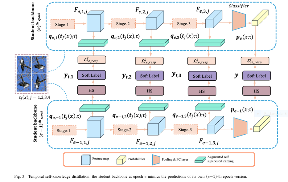
| α | Weight for past‑epoch soft targets | 0.8 |
| β | Balance between label‑supervised and self‑supervised loss | 0.1 |
| γ | Weight for feature‑consistency loss | 0.1 |
Selecting suboptimal values can lead to under‑ or over‑softening, impairing convergence. A robust validation split and grid search are essential to harness LSSKD’s full potential.
8. Best Practices for Implementing LSSKD
To maximize benefits and mitigate drawbacks, follow these tips:
- Start Simple:
- Begin with a single auxiliary classifier at mid‑network depth before scaling to all stages.
- Progressive Tuning:
- First tune α for soft‑label quality, then adjust β/γ for auxiliary losses.
- Data Augmentation:
- Pair LSSKD with CutMix or Cutout for even greater gains (up to +2.58% extra on CIFAR‑100).
- Monitor Compute:
- Benchmark training GPU hours; if overhead is prohibitive, consider pruning seldom‑used auxiliary branches.
- Modality‑Specific Extensions:
- For audio, radar, or text inputs, design SAD transformations tailored to each sensor type.
9. Real‑World Use Cases
LSSKD’s lightweight yet powerful models enable:
- Wearable Health Monitors: Real‑time anomaly detection under power constraints.
- Smart Surveillance Cameras: On‑device person re‑identification with privacy preservation.
- Autonomous Drones: Low‑latency object tracking without cloud offloading.
- Industrial IoT: Predictive maintenance using multimodal sensor fusion at the edge.
In each scenario, LSSKD’s compact student models deliver fast, reliable inference where connectivity is intermittent or bandwidth is limited.
If you’re Interested in more advanced Knowledge Distillation model, you may also find this article helpful: 7 Proven Knowledge Distillation Techniques: Why PLD Outperforms KD and DIST [2025 Update]
Conclusion & Call‑to‑Action
Layered Self‑Supervised Knowledge Distillation offers a powerful yet nuanced path for compressing deep models into edge-friendly champions. By embracing hierarchical label softening and cross‑layer transfer, you can unlock:
- Superior accuracy on tiny models
- Zero inference overhead for real‑time applications
- Robust generalization under scarce data
—but be mindful of the training complexity and hyperparameter tuning required.
Ready to transform your edge AI workflow?
- Download our sample PyTorch implementation of LSSKD today.
- Download Paper for further reading: A Layered Self-Supervised Knowledge Distillation Framework for Efficient Multimodal Learning on the Edge
- Join our community forum to share tips on hyperparameter tuning.
- Subscribe to our newsletter for the latest research on self‑supervised learning and model compression.
Empower your edge devices with the incredible efficiency of LSSKD—where performance meets practicality!
Below is the complete PyTorch implementation of the Layered Self-Supervised Knowledge Distillation (LSSKD) framework. The code includes the model architecture, auxiliary classifiers, self-supervised rotation tasks, and the distillation losses as described in the paper.
import torch
import torch.nn as nn
import torch.nn.functional as F
from torchvision.models import resnet18

class AuxiliaryClassifier(nn.Module):
    """Auxiliary classifier with feature extraction module"""
    def __init__(self, in_channels, num_classes, feat_dim=512):
        super().__init__()
        self.feature_extractor = nn.Sequential(
            nn.Conv2d(in_channels, feat_dim, kernel_size=1),
            nn.BatchNorm2d(feat_dim),
            nn.ReLU(inplace=True)
        )
        self.pool = nn.AdaptiveAvgPool2d(1)
        self.fc = nn.Linear(feat_dim, num_classes)

    def forward(self, x):
        features = self.feature_extractor(x)
        pooled = self.pool(features).flatten(1)
        logits = self.fc(pooled)
        return logits, pooled

class LSSKD_Student(nn.Module):
    def __init__(self, base_model, num_classes, num_rotations=4):
        super().__init__()
        self.backbone = base_model
        self.num_rotations = num_rotations
        self.joint_classes = num_classes * num_rotations

        # Remove original classifier
        if hasattr(self.backbone, 'fc'):
            in_features = self.backbone.fc.in_features
            self.backbone.fc = nn.Identity()
        else:
            in_features = 512  # Default for ResNet variants

        # Final classifier for original task
        self.final_classifier = nn.Linear(in_features, num_classes)

        # Intermediate feature channels for auxiliary classifiers
        self.stage_channels = {
            'layer1': 64,
            'layer2': 128,
            'layer3': 256,
            'layer4': 512
        }

        # Create auxiliary classifiers
        self.aux_classifiers = nn.ModuleDict()
        for name, channels in self.stage_channels.items():
            self.aux_classifiers[name] = AuxiliaryClassifier(
                channels, self.joint_classes
            )

    def forward(self, x, return_features=False):
        # Initial layers
        x = self.backbone.conv1(x)
        x = self.backbone.bn1(x)
        x = self.backbone.relu(x)
        x = self.backbone.maxpool(x)

        # Intermediate features
        features = {}
        x1 = self.backbone.layer1(x)
        features['layer1'] = x1
        x2 = self.backbone.layer2(x1)
        features['layer2'] = x2
        x3 = self.backbone.layer3(x2)
        features['layer3'] = x3
        x4 = self.backbone.layer4(x3)
        features['layer4'] = x4

        # Final features
        pooled_final = self.backbone.avgpool(x4)
        pooled_final = torch.flatten(pooled_final, 1)
        logits_final = self.final_classifier(pooled_final)

        # Auxiliary outputs
        aux_logits = {}
        aux_pooled = {}
        for name, module in self.aux_classifiers.items():
            logits, pooled = module(features[name])
            aux_logits[name] = logits
            aux_pooled[name] = pooled

        if return_features:
            return logits_final, aux_logits, aux_pooled, pooled_final
        return logits_final, aux_logits

def apply_rotation(x, rotation):
    """Apply rotation transformation to batch"""
    if rotation == 0:
        return x
    return torch.rot90(x, k=rotation//90, dims=[2,3])

def lsskd_loss(student_current, student_prev, x, y, alpha=0.8, beta=0.1, gamma=0.1):
    rotations = [0, 90, 180, 270]
    num_rotations = len(rotations)
    batch_size = x.size(0)

    # Create rotated versions
    x_rot = torch.cat([apply_rotation(x, r) for r in rotations], dim=0)
    y_orig = y.repeat(num_rotations)
    rotation_labels = torch.tensor(
        [r_idx for _ in range(batch_size) for r_idx in range(num_rotations)],
        device=x.device
    )
    joint_labels = y_orig * num_rotations + rotation_labels

    # Get predictions from previous model
    with torch.no_grad():
        logits_final_prev, aux_logits_prev, aux_pooled_prev, pooled_final_prev = student_prev(
            x_rot, return_features=True
        )
        p_prev_final = F.softmax(logits_final_prev, dim=1)
        aux_p_prev = {k: F.softmax(v, dim=1) for k, v in aux_logits_prev.items()}

    # Get current predictions
    logits_final_current, aux_logits_current, aux_pooled_current, pooled_final_current = student_current(
        x_rot, return_features=True
    )

    # 1. Responsive CE Loss (Final classifier)
    one_hot_final = F.one_hot(y_orig, num_classes=logits_final_current.size(1)).float()
    soft_target_final = (1 - alpha) * one_hot_final + alpha * p_prev_final
    loss_ce_resp = F.cross_entropy(logits_final_current, soft_target_final)

    # 2. Hierarchical CE Loss (Auxiliary classifiers)
    loss_ce_heir_sad = 0
    num_aux = len(student_current.aux_classifiers)
    for stage in student_current.aux_classifiers:
        one_hot_joint = F.one_hot(joint_labels, num_classes=student_current.joint_classes).float()
        soft_target_aux = (1 - alpha) * one_hot_joint + alpha * aux_p_prev[stage]
        loss_ce_heir_sad += F.cross_entropy(aux_logits_current[stage], soft_target_aux)

    # 3. KL Divergence Loss (Deep to shallow)
    loss_div_sad = 0
    if num_aux > 1:
        # Use last stage as teacher
        teacher_logits = aux_logits_current['layer4']
        for stage in list(student_current.aux_classifiers.keys())[:-1]:
            student_logits = aux_logits_current[stage]
            p_teacher = F.softmax(teacher_logits.detach(), dim=1)
            p_student = F.log_softmax(student_logits, dim=1)
            loss_div_sad += F.kl_div(p_student, p_teacher, reduction='batchmean')

    # 4. Feature L2 Loss
    loss_feat = 0
    for stage in student_current.aux_classifiers:
        # Compare intermediate features to final features
        loss_feat += F.mse_loss(aux_pooled_current[stage], pooled_final_current)

    # Combine losses
    loss_ls = loss_ce_resp + loss_ce_heir_sad
    loss_is = loss_div_sad + loss_feat
    total_loss = (1 - beta) * loss_ls + beta * loss_div_sad + gamma * loss_feat

    return total_loss

# Example usage
if __name__ == "__main__":
    # Initialize models
    num_classes = 100
    base_student = resnet18(pretrained=False)
    student = LSSKD_Student(base_student, num_classes)
    student_prev = LSSKD_Student(resnet18(pretrained=False), num_classes)

    # Dummy data
    x = torch.randn(32, 3, 32, 32)
    y = torch.randint(0, num_classes, (32,))

    # Training step
    optimizer = torch.optim.SGD(student.parameters(), lr=0.05, momentum=0.9, weight_decay=5e-5)
    loss = lsskd_loss(student, student_prev, x, y)

    optimizer.zero_grad()
    loss.backward()
    optimizer.step()

    # After epoch: update previous model
    student_prev.load_state_dict(student.state_dict())

    # For inference: use only final classifier
    logits, _ = student(x)
    print("Final output shape:", logits.shape)
Pingback: Unlock 13% Better Speech Recognition: How Label-Context-Dependent ILM Estimation Shatters CTC Limits - aitrendblend.com