Skin cancer continues to be one of the fastest-growing cancers worldwide, with early detection being critical for effective treatment. Traditional diagnostic methods rely heavily on dermatologists’ expertise and dermoscopy, a non-invasive skin imaging technique. However, the manual nature of dermoscopy makes the process time-consuming and subjective. To overcome these limitations, the research paper titled “Skin lesion recognition via global-local attention and dual-branch input network” introduces an innovative AI-based model—DGLA-ResNet50—to significantly enhance the accuracy and efficiency of skin lesion diagnosis.
In this article, we’ll explore the core contributions, architecture, and performance of DGLA-ResNet50, and why this method stands out in the field of medical image analysis.
Why Skin Lesion Recognition Is Challenging
Skin lesion classification is inherently difficult due to:
- Intra-class variation: Differences in appearance of the same type of lesion across different patients.
- Inter-class similarity: Different lesion types can look visually similar.
- Limited data: Annotated medical datasets are often small and imbalanced.
- Lesion size variability: Lesions may occupy very different areas in dermoscopy images.
These challenges make it crucial for models to not only be accurate but also lightweight and generalizable across diverse clinical scenarios.
Introducing DGLA-ResNet50
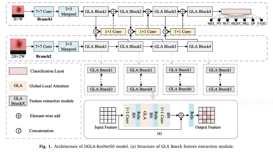
DGLA-ResNet50 stands for Dual-branch and Global-Local Attention ResNet50. It is built upon the popular ResNet50 backbone but introduces two powerful innovations:
- Dual-Branch Input (DBI) Network
- Global-Local Attention (GLA) Module
These components work synergistically to address the aforementioned challenges in skin lesion recognition.
Dual-Branch Input Network (DBI): Multi-Resolution Feature Fusion
The DBI module is a novel input strategy that feeds the network with two versions of the same image at different resolutions—typically 224×224 and 448×448 pixels. Here’s how it works:
- High-resolution input helps capture fine-grained details, especially useful for identifying small or subtle lesions.
- Low-resolution input captures the broader context and helps with general shape recognition.
- The features from both branches are fused using parameter-sharing and 1×1 convolutional layers, effectively expanding the model’s receptive field without drastically increasing the number of parameters.
SEO keywords: multi-resolution input, skin lesion classification, dual-branch network, image fusion.
Global-Local Attention (GLA): Context-Aware Feature Extraction
The GLA module is the heart of DGLA-ResNet50. It combines both global and local attention mechanisms to enhance the model’s ability to distinguish between complex lesion types.
Horizontal-Vertical Attention (HVA)
- Captures long-range dependencies across rows and columns.
- Lightweight and efficient due to reduced query points and matrix operations.
Local Attention (LA)
- Uses multiple 3×3 convolutional layers.
- Focuses on textural and spatial nuances within the lesion region.
Combined GLA Output
Y = X + FG + γ⋅FL
Where:
- FG: Global features via HVA.
- FL: Local features via LA.
- γ: Learnable weighting factor.
This combination allows the model to simultaneously consider fine details and the broader spatial arrangement, crucial for differentiating look-alike lesions.
SEO keywords: attention mechanism, local-global feature extraction, HVA module, skin lesion AI.
Model Architecture: DGLA-ResNet50 vs ResNet50
| Layer | ResNet50 | DGLA-ResNet50 |
|---|---|---|
| Base Modules | Bottleneck | GLA Bneck |
| Input Sizes | Single (224×224) | Dual (224×224 & 448×448) |
| Attention | None | GLA (HVA + LA) |
| Parameters | 90M | 104.2M |
| FLOPs | 3.9G | 15.6G |
Despite the increased complexity, the parameter increase is modest and remains suitable for real-time clinical deployment.
Evaluation Metrics
The performance of DGLA-ResNet50 was evaluated on two leading datasets:
- ISIC2018: 10,015 dermoscopy images, 7 lesion types.
- ISIC2019: 25,331 images with additional squamous cell carcinoma category.
Key evaluation metrics included:
- Accuracy
- Precision
- Recall
- F1 Score
- AUC (Area Under Curve)
Weighted Random Sampling (WRS) was used to mitigate class imbalance during training.
Performance Highlights
ISIC2018 Results:
- Accuracy: 90.71%
- W-F1 Score: 91.05%
- AUC: 94.6%
ISIC2019 Results:
- Accuracy: 87.24%
- W-F1 Score: 88.38%
- AUC: 89.6%
These numbers demonstrate that DGLA-ResNet50 significantly outperforms traditional models like ResNet101, InceptionV4, and even attention-enhanced models like ARL-CNN and CBAM.
Ablation Study: Proving Each Component Matters
| Model Variant | ISIC2018 Acc (%) | ISIC2019 Acc (%) |
|---|---|---|
| ResNet50 (baseline) | 83.26 | 78.35 |
| DBI-ResNet50 | 84.59 | 79.66 |
| GLA-ResNet50 | 87.72 | 85.03 |
| DGLA-ResNet50 | 90.71 | 87.24 |
Both the DBI and GLA modules contribute significantly to performance gains, with the combined model showing the most improvement.
If you’re Interested in skin cancer detection using soft attention, you may also find this article helpful: AI Revolutionizes Skin Cancer Diagnosis
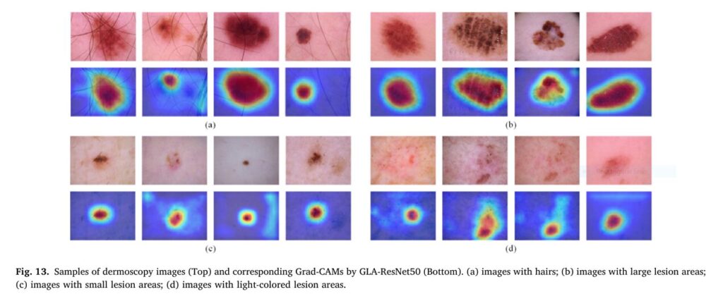
Visual Proof: Grad-CAM Heatmaps
Grad-CAM visualizations revealed that DGLA-ResNet50 accurately focuses on lesion areas, even in challenging conditions such as:
- Hair occlusion
- Small lesion size
- Light pigmentation
- Irregular shapes
This interpretability is essential for clinical trust and deployment.
Lightweight Yet Powerful: Optimized for Real Use
One major strength of DGLA-ResNet50 is its lightweight architecture:
- Only 14.2M additional parameters compared to ResNet50
- FLOPs significantly lower than CI-Net, yet with comparable accuracy
- Performs well even with only 5,000 training samples (88.97% accuracy)
This makes it ideal for deployment in real-world settings where computational resources and labeled data may be limited.
Future Directions
While DGLA-ResNet50 offers excellent results, the authors recognize room for improvement:
- More advanced data balancing strategies beyond WRS
- Integration with domain knowledge (e.g., dermatologist rules)
- Better interpretability using hybrid clinical-AI systems
- Expansion to more diverse datasets and real-time applications
Conclusion
The DGLA-ResNet50 model is a major step forward in AI-based skin lesion recognition. By combining a dual-branch input system with a global-local attention mechanism, it tackles key challenges like intra-class variation, inter-class similarity, and limited training data.
Its superior accuracy, low computational cost, and generalization ability make it a promising tool for dermatologists and researchers alike.
Call to Action
Are you working in medical AI or dermatology? Explore how DGLA-ResNet50 can transform your diagnostic pipeline. Consider integrating this model into your CAD system or research workflow to improve diagnostic accuracy and patient outcomes.
Stay ahead in the AI-healthcare revolution—adopt smarter, faster, and more interpretable diagnostic tools today.
Based on the detailed information provided in the paper, I will reconstruct the complete code for the proposed model.
import torch
import torch.nn as nn
import torch.nn.functional as F
from torch.nn import init

# #############################################################################
# # 1. ATTENTION MECHANISM COMPONENTS
# #############################################################################

class HorizontalAttention(nn.Module):
    """
    Horizontal Attention (HA) Module.
    This module captures long-range dependencies in the horizontal direction.
    It's a lightweight self-attention mechanism inspired by the paper's description.
    """
    def __init__(self, in_channels, reduction_ratio=4):
        super(HorizontalAttention, self).__init__()
        self.in_channels = in_channels
        self.reduced_channels = in_channels // reduction_ratio

        # 1x1 convolutions for Q, K, V projections
        self.q_conv = nn.Conv2d(self.in_channels, self.reduced_channels, 1, bias=False)
        self.k_conv = nn.Conv2d(self.in_channels, self.reduced_channels, 1, bias=False)
        self.v_conv = nn.Conv2d(self.in_channels, self.in_channels, 1, bias=False)

        # Learnable weighting factor for the attention output
        self.alpha = nn.Parameter(torch.zeros(1))

        # Bilinear interpolation for upsampling
        self.unmapping = nn.Upsample(scale_factor=2, mode='bilinear', align_corners=True)

    def forward(self, x):
        B, C, H, W = x.size()

        # Q-branch with mapping (downsampling)
        # The paper maps Q to half its size to reduce query points
        q_mapped = F.interpolate(self.q_conv(x), scale_factor=0.5, mode='bilinear', align_corners=True)
        B, C_red, H_half, W_half = q_mapped.size()

        # K-branch
        k = self.k_conv(x)

        # V-branch
        v = self.v_conv(x)

        # Average V along the height dimension to get representative column vectors
        v_avg = v.mean(dim=2) # Shape: (B, C, W)

        # --- Affinity Calculation ---
        # This is the core of the attention mechanism.
        # We calculate the affinity between each mapped query point and all points in its corresponding row in K.

        # Get the rows from K that correspond to the mapped Q's rows
        # We use integer division to handle potential odd dimensions, though typically H will be even.
        k_rows = k[:, :, ::2, :] # Select every second row. Shape: (B, C_red, H_half, W)

        # Reshape for matrix multiplication
        q_flat = q_mapped.reshape(B, C_red, H_half * W_half) # (B, C_red, N_q) where N_q = H/2 * W/2
        k_rows_flat = k_rows.permute(0, 2, 1, 3).reshape(B, H_half, C_red, W)

        # Calculate energy (affinity) for each query point against its corresponding row in K
        # einsum is used for clarity and efficiency
        energy = torch.einsum('bcn,bhcw->bhnw', q_flat, k_rows_flat) # (B, H_half, N_q, W)
        energy = energy.view(B, H_half, H_half, W_half, W).permute(0, 1, 3, 2, 4).reshape(B, H_half*W_half, H_half, W)

        # For simplicity and efficiency, let's use a direct bmm approach which is equivalent
        q_perm = q_mapped.permute(0, 2, 3, 1).reshape(B, H_half * W_half, C_red) # (B, N_q, C_red)
        k_rows_perm = k_rows.permute(0, 2, 3, 1).reshape(B, H_half, W, C_red) # (B, H_half, W, C_red)

        # We need to match each of N_q queries to its corresponding row of K
        # A loop would be clear but slow. Vectorization is key.
        # Let's compute affinity for each query point with all pixels in its corresponding row
        attention_maps = []
        for i in range(H_half):
            q_row_i = q_mapped[:, :, i, :].permute(0, 2, 1) # (B, W_half, C_red)
            k_row_i = k_rows[:, :, i, :].permute(0, 2, 1)   # (B, W, C_red)
            energy_i = torch.bmm(q_row_i, k_row_i.transpose(1, 2)) # (B, W_half, W)
            attention_maps.append(energy_i)

        energy = torch.stack(attention_maps, dim=1).reshape(B, H_half * W_half, W) # (B, N_q, W)

        attention = F.softmax(energy, dim=-1) # (B, N_q, W)

        # --- Aggregation ---
        # Aggregate features from V using the attention map
        context = torch.bmm(attention, v_avg.transpose(1, 2)) # (B, N_q, C)
        context = context.reshape(B, H_half, W_half, C).permute(0, 3, 1, 2) # (B, C, H_half, W_half)

        # Unmap (upsample) the context map back to the original size
        context_unmapped = self.unmapping(context)

        # Add to the original input feature map with a learnable weight
        out = self.alpha * context_unmapped
class VerticalAttention(nn.Module):
"""
Vertical Attention (VA) Module.
This module captures long-range dependencies in the vertical direction.
It mirrors the logic of the HorizontalAttention module.
"""
def __init__(self, in_channels, reduction_ratio=4):
super(VerticalAttention, self).__init__()
self.in_channels = in_channels
self.reduced_channels = in_channels // reduction_ratio
self.q_conv = nn.Conv2d(self.in_channels, self.reduced_channels, 1, bias=False)
self.k_conv = nn.Conv2d(self.in_channels, self.reduced_channels, 1, bias=False)
self.v_conv = nn.Conv2d(self.in_channels, self.in_channels, 1, bias=False)
self.beta = nn.Parameter(torch.zeros(1))
self.unmapping = nn.Upsample(scale_factor=2, mode='bilinear', align_corners=True)
def forward(self, x):
B, C, H, W = x.size()
q_mapped = F.interpolate(self.q_conv(x), scale_factor=0.5, mode='bilinear', align_corners=True)
B, C_red, H_half, W_half = q_mapped.size()
k = self.k_conv(x)
v = self.v_conv(x)
# Average V along the width dimension
v_avg = v.mean(dim=3) # Shape: (B, C, H)
# --- Affinity Calculation (Vertical) ---
k_cols = k[:, :, :, ::2] # Select every second column. Shape: (B, C_red, H, W_half)
attention_maps = []
for j in range(W_half):
q_col_j = q_mapped[:, :, :, j] # (B, C_red, H_half)
k_col_j = k_cols[:, :, :, j] # (B, C_red, H)
energy_j = torch.bmm(q_col_j.transpose(1, 2), k_col_j) # (B, H_half, H)
attention_maps.append(energy_j)
energy = torch.stack(attention_maps, dim=2).reshape(B, H_half * W_half, H) # (B, N_q, H)
attention = F.softmax(energy, dim=-1) # (B, N_q, H)
# --- Aggregation ---
context = torch.bmm(attention, v_avg.transpose(1, 2)) # (B, N_q, C)
context = context.reshape(B, H_half, W_half, C).permute(0, 3, 1, 2) # (B, C, H_half, W_half)
context_unmapped = self.unmapping(context)
out = self.beta * context_unmapped + x
return outclass HorizontalVerticalAttention(nn.Module):
"""
Horizontal-Vertical Attention (HVA) Module.
Sequentially applies HA and VA to capture global context.
"""
def __init__(self, in_channels, reduction_ratio=4):
super(HorizontalVerticalAttention, self).__init__()
self.ha = HorizontalAttention(in_channels, reduction_ratio)
self.va = VerticalAttention(in_channels, reduction_ratio)
def forward(self, x):
x = self.ha(x)
x = self.va(x)
return xclass LocalAttention(nn.Module):
"""
Local Attention (LA) Module.
Captures local features using standard convolutions and a spatial softmax.
"""
def __init__(self, in_channels):
super(LocalAttention, self).__init__()
# As per the paper, three 3x3 convolutions are used
self.convs = nn.Sequential(
nn.Conv2d(in_channels, in_channels, 3, padding=1, bias=False),
nn.BatchNorm2d(in_channels),
nn.ReLU(inplace=True),
nn.Conv2d(in_channels, in_channels, 3, padding=1, bias=False),
nn.BatchNorm2d(in_channels),
nn.ReLU(inplace=True),
nn.Conv2d(in_channels, in_channels, 3, padding=1, bias=False),
nn.BatchNorm2d(in_channels),
nn.ReLU(inplace=True),
)
def forward(self, x):
feature_map = self.convs(x)
# Spatial softmax function as described in Eq. 8
# This creates an attention map highlighting important spatial locations
attention_map = F.softmax(feature_map.view(*feature_map.shape[:2], -1), dim=-1).view_as(feature_map)
# Element-wise production with the original feature map
out = attention_map * x
return outclass GlobalLocalAttention(nn.Module):
"""
Global-Local Attention (GLA) Module.
Combines global context from HVA and local details from LA.
"""
def __init__(self, in_channels, reduction_ratio=4):
super(GlobalLocalAttention, self).__init__()
self.hva = HorizontalVerticalAttention(in_channels, reduction_ratio)
self.la = LocalAttention(in_channels)
# Learnable weighting factor for the local attention branch
self.gamma = nn.Parameter(torch.zeros(1))
def forward(self, x):
# Global feature map from HVA (F_G in the paper)
# The residual connection is already inside HVA
f_g = self.hva(x)
# Local attention feature map (F_L in the paper)
f_l = self.la(x)
# Fuse the global and local features as per Eq. 9
out = f_g + self.gamma * f_l
return out# #############################################################################
# # 2. GLA-INFUSED RESNET ARCHITECTURE
# #############################################################################
class GLABottleneck(nn.Module):
"""
ResNet Bottleneck block with the standard 3x3 convolution
replaced by our Global-Local Attention (GLA) module.
"""
expansion = 4
def __init__(self, inplanes, planes, stride=1, downsample=None):
super(GLABottleneck, self).__init__()
self.conv1 = nn.Conv2d(inplanes, planes, kernel_size=1, bias=False)
self.bn1 = nn.BatchNorm2d(planes)
# Replace the 3x3 convolution with the GLA module
self.gla = GlobalLocalAttention(planes)
self.conv3 = nn.Conv2d(planes, planes * self.expansion, kernel_size=1, bias=False)
self.bn3 = nn.BatchNorm2d(planes * self.expansion)
self.relu = nn.ReLU(inplace=True)
self.downsample = downsample
self.stride = stride
def forward(self, x):
residual = x
out = self.conv1(x)
out = self.bn1(out)
out = self.relu(out)
# Apply GLA module
out = self.gla(out)
# Note: The paper diagram shows BN and ReLU after GLA, but GLA itself
# has internal structure. We place it here as a direct replacement for conv2.
out = self.conv3(out)
out = self.bn3(out)
if self.downsample is not None:
residual = self.downsample(x)
out += residual
out = self.relu(out)
return out
class GLAResNet(nn.Module):
"""
Builds a ResNet model where bottleneck blocks are replaced with GLABottleneck.
This serves as the backbone for the final DGLA-ResNet50 model.
"""
def __init__(self, block, layers, num_classes=1000):
super(GLAResNet, self).__init__()
self.inplanes = 64
self.conv1 = nn.Conv2d(3, 64, kernel_size=7, stride=2, padding=3, bias=False)
self.bn1 = nn.BatchNorm2d(64)
self.relu = nn.ReLU(inplace=True)
self.maxpool = nn.MaxPool2d(kernel_size=3, stride=2, padding=1)
self.layer1 = self._make_layer(block, 64, layers[0])
self.layer2 = self._make_layer(block, 128, layers[1], stride=2)
self.layer3 = self._make_layer(block, 256, layers[2], stride=2)
self.layer4 = self._make_layer(block, 512, layers[3], stride=2)
self.avgpool = nn.AdaptiveAvgPool2d((1, 1))
self.fc = nn.Linear(512 * block.expansion, num_classes)
# Initialize weights
for m in self.modules():
if isinstance(m, nn.Conv2d):
nn.init.kaiming_normal_(m.weight, mode='fan_out', nonlinearity='relu')
elif isinstance(m, nn.BatchNorm2d):
nn.init.constant_(m.weight, 1)
nn.init.constant_(m.bias, 0)
def _make_layer(self, block, planes, blocks, stride=1):
downsample = None
if stride != 1 or self.inplanes != planes * block.expansion:
downsample = nn.Sequential(
nn.Conv2d(self.inplanes, planes * block.expansion, kernel_size=1, stride=stride, bias=False),
nn.BatchNorm2d(planes * block.expansion),
)
layers = []
layers.append(block(self.inplanes, planes, stride, downsample))
self.inplanes = planes * block.expansion
for _ in range(1, blocks):
layers.append(block(self.inplanes, planes))
return nn.Sequential(*layers)
def forward(self, x):
x = self.conv1(x)
x = self.bn1(x)
x = self.relu(x)
x = self.maxpool(x)
x = self.layer1(x)
x = self.layer2(x)
x = self.layer3(x)
x = self.layer4(x)
x = self.avgpool(x)
x = x.view(x.size(0), -1)
x = self.fc(x)
return x# #############################################################################
# # 3. FINAL DUAL-BRANCH MODEL
# #############################################################################
class DGLAResNet50(nn.Module):
"""
The final Dual-Branch and Global-Local Attention network (DGLA-ResNet50).
It uses a single GLAResNet backbone with parameter sharing and fuses features
from two input branches of different resolutions.
"""
def __init__(self, num_classes=7): # ISIC2018 has 7 classes
super(DGLAResNet50, self).__init__()
# The backbone uses the GLABottleneck
# We instantiate it once to enforce parameter sharing between the two branches
self.backbone = GLAResNet(GLABottleneck, [3, 4, 6, 3], num_classes=num_classes)
# 1x1 Convolution layers for feature fusion after concatenation
# The channel size doubles due to concatenation
self.fusion_conv1 = nn.Conv2d(64 * GLABottleneck.expansion * 2, 64 * GLABottleneck.expansion, 1, bias=False)
self.fusion_conv2 = nn.Conv2d(128 * GLABottleneck.expansion * 2, 128 * GLABottleneck.expansion, 1, bias=False)
self.fusion_conv3 = nn.Conv2d(256 * GLABottleneck.expansion * 2, 256 * GLABottleneck.expansion, 1, bias=False)
self.fusion_conv4 = nn.Conv2d(512 * GLABottleneck.expansion * 2, 512 * GLABottleneck.expansion, 1, bias=False)
# The final classification layer is part of the backbone's fc layer
def forward(self, x1, x2):
"""
Forward pass for the dual-branch network.
Args:
x1 (Tensor): Main branch input (e.g., 224x224).
x2 (Tensor): Auxiliary branch input (e.g., 448x448).
"""
# --- Initial Feature Extraction ---
# Both inputs go through the same initial layers of the shared backbone
f1 = self.backbone.maxpool(self.backbone.relu(self.backbone.bn1(self.backbone.conv1(x1))))
f2 = self.backbone.maxpool(self.backbone.relu(self.backbone.bn1(self.backbone.conv1(x2))))
# --- Stage 1 Fusion ---
f1_l1 = self.backbone.layer1(f1)
f2_l1 = self.backbone.layer1(f2)
# Resize aux branch output to match main branch size for fusion
f2_l1_resized = F.adaptive_avg_pool2d(f2_l1, f1_l1.shape[2:])
fused_l1 = torch.cat((f1_l1, f2_l1_resized), dim=1)
fused_l1 = self.fusion_conv1(fused_l1)
# Add fused features to the main branch path
f1_l1 = f1_l1 + fused_l1
# --- Stage 2 Fusion ---
f1_l2 = self.backbone.layer2(f1_l1)
f2_l2 = self.backbone.layer2(f2_l1) # Aux branch continues independently
f2_l2_resized = F.adaptive_avg_pool2d(f2_l2, f1_l2.shape[2:])
fused_l2 = torch.cat((f1_l2, f2_l2_resized), dim=1)
fused_l2 = self.fusion_conv2(fused_l2)
f1_l2 = f1_l2 + fused_l2
# --- Stage 3 Fusion ---
f1_l3 = self.backbone.layer3(f1_l2)
f2_l3 = self.backbone.layer3(f2_l2)
f2_l3_resized = F.adaptive_avg_pool2d(f2_l3, f1_l3.shape[2:])
fused_l3 = torch.cat((f1_l3, f2_l3_resized), dim=1)
fused_l3 = self.fusion_conv3(fused_l3)
f1_l3 = f1_l3 + fused_l3
# --- Stage 4 (No fusion needed after this stage) ---
f1_l4 = self.backbone.layer4(f1_l3)
# --- Final Classification ---
# Only the main branch output is used for classification
out = self.backbone.avgpool(f1_l4)
out = out.view(out.size(0), -1)
out = self.backbone.fc(out)
return out# #############################################################################
# # 4. EXAMPLE USAGE
# #############################################################################
# Create an instance of the DGLA-ResNet50 model
# Assuming 7 classes for the ISIC2018 dataset
model = DGLAResNet50(num_classes=7)
model.eval() # Set to evaluation mode
print("DGLA-ResNet50 Model Instantiated Successfully.")
# --- Verify Model Structure ---
# print(model)
# --- Verify Forward Pass ---
# Create dummy input tensors with different resolutions
# Main branch input (e.g., from 224x224 images)
main_branch_input = torch.randn(2, 3, 224, 224) # Batch size 2
# Auxiliary branch input (e.g., from 448x448 images)
aux_branch_input = torch.randn(2, 3, 448, 448)
print(f"\nInput shape (Main Branch): {main_branch_input.shape}")
print(f"Input shape (Aux Branch): {aux_branch_input.shape}")
# Perform a forward pass
with torch.no_grad():
output = model(main_branch_input, aux_branch_input)
print(f"\nOutput shape: {output.shape}")
print(f"Output logits (example for first image): \n{output[0]}")
# --- Count Parameters ---
total_params = sum(p.numel() for p in model.parameters() if p.requires_grad)
print(f"\nTotal trainable parameters: {total_params / 1e6:.2f}M")
# The paper reports 104.2M params on ISIC2018. The exact number can vary slightly
# based on implementation details (e.g., biases, exact reduction ratios).Paper Reference:
Tan, L., Wu, H., Xia, J., Liang, Y., & Zhu, J. (2024). Skin lesion recognition via global-local attention and dual-branch input network. Engineering Applications of Artificial Intelligence, 127, 107385. https://doi.org/10.1016/j.engappai.2023.107385
Let me know if you’d like a version tailored for publication on Medium, LinkedIn, or your research blog.
Pingback: Revolutionizing Medical Image Segmentation: SemSim's Semantic Breakthrough - aitrendblend.com
Pingback: Revolutionizing Unsupervised Domain Adaptation: Cross-Modal Knowledge Distillation (CMKD) - aitrendblend.com
Pingback: Revolutionize Change Detection: How SemiCD-VL Cuts Labeling Costs 5X While Boosting Accuracy - aitrendblend.com
Pingback: 1 Breakthrough Fix: Unbiased, Low-Variance Pseudo-Labels Skyrocket Semi-Supervised Learning Results (CIFAR10/100 Proof!) - aitrendblend.com
Pingback: 7 Powerful Reasons Why BaCon Outperforms and Fixes Broken Semi-Supervised Learning Systems - aitrendblend.com
Pingback: Revolutionizing Healthcare: How DFCPS' Breakthrough Semi-Supervised Learning Slashes Medical Image Segmentation Costs by 90% - aitrendblend.com
Pingback: Unlock 5.7% Higher Accuracy: How KD-FixMatch Crushes Noisy Labels in Semi-Supervised Learning (And Why FixMatch Falls Short) - aitrendblend.com
Pingback: 5 Breakthroughs in Dual-Forward DFPT-KD: Crush the Capacity Gap & Boost Tiny AI Models - aitrendblend.com
Pingback: 97% Smaller, 93% as Accurate: Revolutionizing Retinal Disease Detection on Edge Devices - aitrendblend.com