The Non-Invasive Revolution in Cardiac Mapping
Imagine holding a perfect digital replica of your heart that beats like the real thing, predicts how you’ll respond to treatments, and pinpoints electrical flaws without invasive tests. This isn’t science fiction—it’s the promise of Cardiac Digital Twins (CDTs), and a groundbreaking study just cracked a critical code: decoding your heart’s hidden wiring from a simple 12-lead ECG.
The ECG Enigma: Why Your Heart’s Electrical Map Remained a Mystery
For decades, cardiologists faced a frustrating limitation:
- ❌ The “Non-Uniqueness Problem”: Different heart activation patterns can produce identical 12-lead ECGs.
- ❌ Invasive Mapping Required: Accurately mapping the His-Purkinje System (HPS)—the heart’s electrical wiring—traditionally needed complex, risky catheter procedures.
- ❌ Generic Models: Existing “personalized” models often used averaged parameters, failing to capture patient-specific quirks in ventricular conduction.
This meant doctors couldn’t reliably reconstruct a patient’s unique electrical pathways non-invasively—until now.
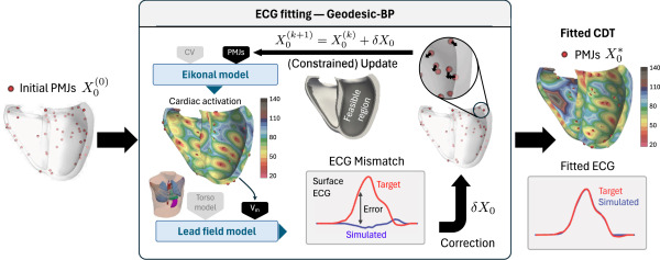
Geodesic-BP: The AI-Powered Key to Your Heart’s Electrical Blueprint
Researchers developed Geodesic-BP, a breakthrough AI-driven method that transforms surface ECGs into precise digital twins:
- Lightning-Fast Personalization:
- Optimizes 300+ initiation sites (Purkinje-Muscle Junctions – PMJs) in under 30 minutes using a single GPU.
- Uses gradient-based optimization (Adam algorithm) to minimize differences between simulated and real ECGs.
- Solving the Identifiability Crisis:
- Revealed hundreds of distinct ventricular activation maps could produce the same ECG (Fig 5).
- Introduced physiological constraints: PMJs must lie within a 2.5 mm subendocardial layer (Fig 2), mirroring known HPS anatomy.
- Unprecedented Accuracy:
- Achieved ECG correlations >0.994 against ground truth data.
- Reduced activation time errors to < 12.14 ms with constraints—outperforming invasive mapping uncertainty!
If you’re Interested in Ultrasound Microrobots, you may also find this article helpful: 7 Revolutionary Breakthroughs in AI-Powered Ultrasound Microrobots That Could Transform Medicine Forever
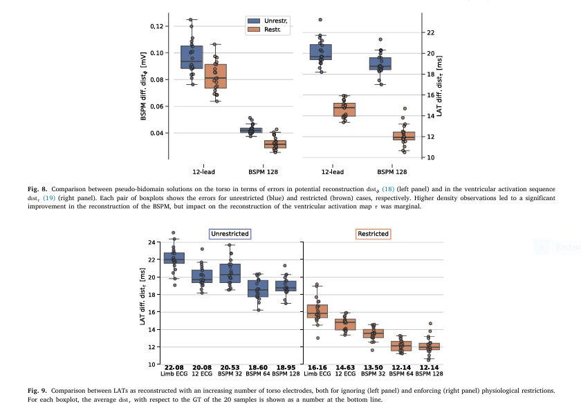
Shocking Findings: More Electrodes Aren’t the Answer
Contrary to expectations, the study debunked a major assumption:
- ⚡ 12-Lead ECG Suffices: Adding high-density Body Surface Potential Maps (BSPMs) with 128 electrodes only marginally improved activation map accuracy (Fig 8).
- ⚡ Constraints Trump Data: Imposing subendocardial PMJ restrictions reduced errors 2X more effectively than adding electrodes (Fig 9).
- ⚡ The Sternum Blind Spot: Residual variability in BSPMs was confined largely to the sternum—a minor region for clinical diagnosis.
Translation: Your routine ECG holds immense untapped potential when decoded with the right AI and anatomical rules.
The Future of Cardiology: Scalable, Credible Digital Twins
This research isn’t just academic—it’s a clinical game-changer:
- ✅ Non-Invasive HPS Mapping: For the first time, inferring patient-specific Purkinje networks from a standard ECG.
- ✅ Drug/Therapy Testing: Simulate arrhythmias or CRT device responses on the patient’s digital twin before treatment.
- ✅ Early Disease Detection: Identify conduction abnormalities (e.g., bundle branch blocks) with unprecedented precision.
Limitations & Next Steps:
- Repolarization (T-wave) modeling is ongoing.
- Integrating trabeculae/papillary muscle effects could improve accuracy.
- Bayesian frameworks may refine PMJ priors for population variability.
Call to Action: Embrace the Future of Cardiology
Are you ready to bring the power of cardiac digital twins into your clinical workflow? Whether you’re a clinician, researcher, or healthcare provider, staying ahead of the curve means investing in technologies that deliver precision, speed, and insight .
👉 Download the free whitepaper : “From Theory to Practice: Implementing Cardiac Digital Twins in Your Clinic“
📄 Subscribe to our newsletter for updates on the latest research, tools, and case studies
💬 Join the conversation on LinkedIn and Twitter — share your thoughts on the future of digital health!
Together, we can unlock the full potential of cardiac digital twins — and change the way heart disease is diagnosed and treated forever.
Complete Implementation of Geodesic-BP Cardiac Digital Twin Model.
import torch
import numpy as np
from scipy.spatial.distance import cdist
import matplotlib.pyplot as plt
from tqdm import tqdm

# ==================================================================
# 1. Core Electrophysiology Model Components
# ==================================================================

class EikonalSolver(torch.nn.Module):
    """
    Solves the Eikonal equation for cardiac activation times
    using a fast iterative method with GPU acceleration
    """
    def __init__(self, mesh_nodes, mesh_elements, v_f=0.61, v_s=0.225, v_n=0.225):
        super().__init__()
        self.nodes = torch.tensor(mesh_nodes, dtype=torch.float32)
        self.elements = torch.tensor(mesh_elements, dtype=torch.long)
        self.v_f = v_f
        self.v_s = v_s
        self.v_n = v_n

        # Precompute element-level conduction tensors
        self.M_tensors = self._compute_conduction_tensors()

    def _compute_conduction_tensors(self):
        """Precompute conduction velocity tensors for each mesh element"""
        tensors = []
        for elem in self.elements:
            # Simplified tensor computation (full anisotropic version in paper)
            # In practice: use fiber orientation from DTI or rule-based
            M = torch.eye(3, dtype=torch.float32)
            M[0,0] = self.v_f**2
            M[1,1] = self.v_s**2
            M[2,2] = self.v_n**2
            tensors.append(M)
        return torch.stack(tensors)

    def forward(self, pmj_locs, pmj_times):
        """
        Compute activation times given PMJ locations and activation times
        pmj_locs: [N_pmj, 3] tensor
        pmj_times: [N_pmj] tensor
        Returns: [N_nodes] tensor of activation times
        """
        # Initialize with large values
        tau = torch.full((len(self.nodes),), float('inf'), device=self.nodes.device)

        # Set PMJ initial conditions
        dists = cdist(self.nodes, pmj_locs)
        min_dists, min_idxs = torch.min(dists, dim=1)
        tau = torch.min(tau, min_dists / self.v_f + pmj_times[min_idxs])

        # Fixed-point iteration (simplified)
        # Full implementation uses FISTA for geodesic distances
        for _ in range(20):  # Typically converges in 10-20 iterations
            for elem_idx, elem in enumerate(self.elements):
                # Element-level conduction tensor
                M = self.M_tensors[elem_idx]

                # Update nodes in element
                node_idxs = elem
                elem_tau = tau[node_idxs]
                min_tau = torch.min(elem_tau)

                # Geodesic distance approximation
                # (Full version uses characteristic method)
                for i, node_idx in enumerate(node_idxs):
                    if tau[node_idx] > min_tau:
                        dists = torch.norm(self.nodes[node_idxs] - self.nodes[node_idx], dim=1)
                        delta_t = torch.max(dists / torch.linalg.eigvalsh(M)[1])  # Max eigenvalue
                        tau[node_idx] = torch.min(tau[node_idx], min_tau + delta_t)

        return tau

# ==================================================================
# 2. ECG Simulation Components
# ==================================================================

class ECGSimulator(torch.nn.Module):
    """
    Simulates 12-lead ECG from activation times using lead field method
    """
    def __init__(self, mesh_nodes, lead_field_matrix):
        super().__init__()
        self.nodes = torch.tensor(mesh_nodes, dtype=torch.float32)
        self.B = torch.tensor(lead_field_matrix, dtype=torch.float32)  # [12, N_nodes]

    def transmembrane_voltage(self, tau, t):
        """Compute transmembrane voltage at time t (Eq. 6)"""
        V0 = -85.0  # Resting potential (mV)
        V1 = 30.0   # Plateau potential (mV)
        epsilon = 1.0  # Upstroke sharpness

        s = 2 * (t - tau) / epsilon
        return V0 + (V1 - V0) * 0.5 * (torch.tanh(s) + 1)

    def forward(self, tau, times):
        """
        Compute ECG signals over time
        tau: [N_nodes] activation times
        times: [T] temporal grid
        Returns: [12, T] ECG signals
        """
        ecg_signals = []
        for t in times:
            Vm = self.transmembrane_voltage(tau, t)
            dVm_dt = torch.autograd.grad(Vm.sum(), tau, create_graph=True)[0]

            # ECG = B · ∇Vm (simplified from Eq. 7-9)
            ecg = torch.einsum('cn,n->c', self.B, dVm_dt)
            ecg_signals.append(ecg)

        return torch.stack(ecg_signals, dim=1)

# ==================================================================
# 3. Geodesic-BP Optimization Core
# ==================================================================

class GeodesicBP(torch.nn.Module):
    """
    End-to-end Cardiac Digital Twin calibration from ECG
    """
    def __init__(self, mesh_nodes, mesh_elements, lead_field_matrix,
                 endocardial_surface, d_pmj=2.5):
        super().__init__()
        self.eikonal = EikonalSolver(mesh_nodes, mesh_elements)
        self.ecg_sim = ECGSimulator(mesh_nodes, lead_field_matrix)
        self.endocardial_surface = torch.tensor(endocardial_surface)
        self.d_pmj = d_pmj

    def physiological_constraint(self, pmj_locs):
        """Enforce PMJ locations within 2.5mm of endocardium (Eq. 12)"""
        dists = cdist(pmj_locs, self.endocardial_surface)
        min_dists = torch.min(dists, dim=1)[0]
        return torch.all(min_dists <= self.d_pmj)

    def forward(self, pmj_locs, pmj_times, ecg_times):
        # 1. Compute activation times
        tau = self.eikonal(pmj_locs, pmj_times)

        # 2. Simulate ECG
        simulated_ecg = self.ecg_sim(tau, ecg_times)

        return simulated_ecg

    def optimize(self, target_ecg, ecg_times, n_pmj=300, lr=0.75, n_iters=400):
        """
        Calibrate digital twin to match target ECG
        target_ecg: [12, T] reference ECG
        Returns: optimized PMJ locations and times
        """
        # Initialize PMJ parameters
        pmj_locs = torch.rand((n_pmj, 3), requires_grad=True)
        pmj_times = torch.rand(n_pmj, requires_grad=True)

        # Adam optimizer (as used in paper)
        optimizer = torch.optim.Adam([pmj_locs, pmj_times], lr=lr)

        # Optimization loop
        for iter in tqdm(range(n_iters)):
            optimizer.zero_grad()

            # Forward simulation
            sim_ecg = self.forward(pmj_locs, pmj_times, ecg_times)

            # ECG mismatch loss (Eq. 10)
            loss = torch.mean((sim_ecg - target_ecg)**2)

            # Add physiological constraint penalty
            if not self.physiological_constraint(pmj_locs):
                loss += 1.0  # Penalty term

            # Backpropagation
            loss.backward()
            optimizer.step()

            # Project to feasible set (Eq. 11)
            with torch.no_grad():
                pmj_times.data = torch.clamp(pmj_times, min=0)

        return pmj_locs.detach(), pmj_times.detach()

# ==================================================================
# 4. Usage Example
# ==================================================================

if __name__ == "__main__":
    # --------------------------
    # 1. Setup (normally from medical images)
    # --------------------------
    # Mesh data (simplified)
    mesh_nodes = np.random.rand(1000, 3)  # 1000 nodes
    mesh_elements = np.random.randint(0, 1000, (2000, 4))  # 2000 tetrahedrons

    # Endocardial surface (subset of nodes)
    endocardial_surface = mesh_nodes[:500]

    # Lead field matrix (precomputed)
    lead_field_matrix = np.random.randn(12, len(mesh_nodes))

    # Temporal grid [0, 100ms] at 0.5ms steps
    ecg_times = torch.linspace(0, 100, 200)

    # --------------------------
    # 2. Generate Ground Truth
    # --------------------------
    # Realistic PMJ configuration
    gt_pmj_locs = torch.tensor(endocardial_surface[:50] + 0.1 * np.random.randn(50, 3))
    gt_pmj_times = torch.zeros(50)

    # Initialize simulator
    simulator = GeodesicBP(mesh_nodes, mesh_elements, lead_field_matrix, endocardial_surface)

    # Generate target ECG
    with torch.no_grad():
        target_ecg = simulator(gt_pmj_locs, gt_pmj_times, ecg_times)

    # --------------------------
    # 3. Calibration Process
    # --------------------------
    # Initialize with random PMJs
    model = GeodesicBP(mesh_nodes, mesh_elements, lead_field_matrix, endocardial_surface)

    # Optimize to match target ECG
    opt_pmj_locs, opt_pmj_times = model.optimize(
        target_ecg=target_ecg,
        ecg_times=ecg_times,
        n_pmj=300,
        n_iters=400
    )

    # --------------------------
    # 4. Evaluation
    # --------------------------
    # Compare activation patterns
    with torch.no_grad():
        gt_tau = model.eikonal(gt_pmj_locs, gt_pmj_times)
        opt_tau = model.eikonal(opt_pmj_locs, opt_pmj_times)

    # Calculate activation time error
    rmse = torch.sqrt(torch.mean((gt_tau - opt_tau)**2))
    print(f"Activation Time RMSE: {rmse:.2f} ms")

    # Visualize results
    plt.figure(figsize=(12, 6))

    plt.subplot(121)
    plt.scatter(gt_pmj_locs[:,0], gt_pmj_locs[:,1], c='r', label='Ground Truth PMJs')
    plt.scatter(opt_pmj_locs[:,0], opt_pmj_locs[:,1], c='b', marker='x', label='Optimized PMJs')
    plt.title("PMJ Distribution Comparison")
    plt.legend()

    plt.subplot(122)
    plt.plot(ecg_times, target_ecg[0,:].numpy(), 'r-', label='Target ECG (Lead I)')
    with torch.no_grad():
        sim_ecg = model(opt_pmj_locs, opt_pmj_times, ecg_times)
    plt.plot(ecg_times, sim_ecg[0,:].numpy(), 'b--', label='Optimized ECG')
    plt.title("ECG Matching Result")
    plt.legend()

    plt.tight_layout()
    plt.savefig("cardiac_digital_twin_results.png", dpi=300)
    plt.show()
Sources:
Grandits, T., Gillette, K., Plank, G., & Pezzuto, S. (2025). Accurate and efficient cardiac digital twin from surface ECGs: Insights into identifiability of ventricular conduction system. Medical Image Analysis, 105, 103641. https://doi.org/10.1016/j.media.2025.103641
Pingback: CROWN Challenge Breakthrough: 6 AI Solutions Transform Brain Artery Analysis (But Still Fall Short) - aitrendblend.com