3 Breakthroughs & 1 Warning: How Explainable AI SVIS-RULEX is Revolutionizing Medical Imaging (Finally!)

For years, artificial intelligence (AI) has promised to revolutionize medical diagnosis, particularly in analyzing complex medical images like X-rays, MRIs, and ultrasounds. Deep learning models consistently achieve superhuman accuracy in spotting tumors, infections, and subtle pathologies. Yet, a critical roadblock remains: the “black box” problem. How does the AI really make its decision? Without transparency, doctors hesitate to trust it, regulators struggle to approve it, and lives potentially hang in the balance.

But a groundbreaking new framework, SVIS-RULEX, is shattering this barrier. Published in Medical Image Analysis (105, 2025), this research delivers a powerful trifecta of interpretability, finally making medical AI trustworthy and actionable. Let’s dive into how it works, why it matters, and the one crucial caveat you need to know.

The Frustrating Black Box Problem in Medical AI

Imagine a sophisticated AI that detects lung cancer in X-rays with 95% accuracy – better than most radiologists. Yet, when asked why it flagged a specific image, it can only shrug (metaphorically). Was it the subtle nodule? The texture? The surrounding tissue? This lack of explanation is more than an academic concern; it’s a critical flaw:

1. Eroded Trust: Clinicians are rightfully skeptical of decisions they cannot understand or verify. Would you base a critical diagnosis or treatment plan on a system you can’t interrogate?
2. Ethical & Regulatory Hurdles: How can we ensure AI isn’t biased? How can we explain errors? Regulatory bodies (like the FDA) demand explainability for approval.
3. Missed Opportunities: Without understanding how the AI works, doctors lose valuable insights that could refine their own diagnostic skills or uncover new biomarkers.
4. Limited Adoption: The “black box” is a primary reason powerful AI tools gather dust instead of saving lives in clinics.

Traditional “Explainable AI” (XAI) methods often fall short in medicine. Saliency maps (like Grad-CAM) highlight “important” regions but don’t explain what features (texture? intensity? shape?) were crucial. Rule-based systems offer clear “if-then” logic but struggle with the complexity of image data. Statistical analyses can be abstract. SVIS-RULEX tackles these limitations head-on by integrating all three.

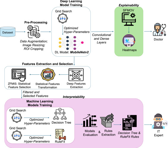
How SVIS-RULEX Cracks Open the Black Box: 3 Integrated Breakthroughs

Developed by Ullah et al., SVIS-RULEX isn’t just one technique; it’s a comprehensive pipeline designed specifically for medical image analysis, combining statistical depth, visual clarity, and rule-based simplicity:

1. From Deep Features to Human-Understandable Stats (The “Why” Behind Pixels):
   • Step 1: A custom, efficient MobileNetV2 model processes the medical image (X-ray, ultrasound, MRI, etc.), extracting complex “deep features” from its layers. These features are powerful but abstract.
   • Step 2: Statistical Feature Engineering: This is the first breakthrough. Instead of relying on cryptic deep features, SVIS-RULEX calculates 26 intuitive statistical measures (like Mean, Variance, Skewness, Entropy, Signal-to-Noise Ratio, Correlation) directly from those deep features or relevant image regions. Think of it as translating AI jargon into the language of medical data analysis.
   • Step 3: Smart Feature Selection (ZFMIS): Not all stats are equally important. A novel two-stage filter (Zero-based Filtering + Mutual Importance Selection) removes irrelevant or noisy features (e.g., those with too many zeros or low predictive power), leaving a potent, interpretable subset. Example Top Features: Harmonic Mean (HM), Skewness (Skew), Coefficient of Variation (CV) were crucial for COVID-19 X-ray classification.
2. Rule-Based Transparency (The “Logic” of Diagnosis):
   • Step 4: Human-Readable Rules: The selected statistical features are fed into inherently interpretable models:
     • Decision Trees (DT): Build hierarchical “if-then” rules based on feature thresholds (e.g., “IF Entropy > 3.92 AND Geometric Mean <= 0.001 THEN Malignant Tumor”).
     • RuleFit: Generates an ensemble of powerful, concise rules, often combining features (e.g., “IF Correlation <= -0.17 AND Coefficient of Variation > 1.26 THEN Colon Benign”). RuleFit balances accuracy with interpretability.
   • Simplification: Raw rules are refined to remove redundancy, presenting clinicians with clear, actionable logic for why a specific class (e.g., COVID, malignant tumor) was predicted. This is the core “explanation” output.
3. Visual Proof with Statistical Overlays (SFMOV – The “Where” and “What”):
   • Step 5: Statistical Feature Map Overlay Visualization (SFMOV): This is the second major breakthrough and the visual cornerstone. SVIS-RULEX doesn’t just show where (like standard heatmaps), it shows what kind of feature matters visually:
     • It calculates localized statistical maps (Mean, Skewness, Entropy) across the image, highlighting areas with specific properties (e.g., high average intensity, asymmetric texture, complex patterns).
     • Crucially, it weights these maps using importance derived from the model’s dense layers.
     • It creates a combined heatmap (H(x,y) = w1*Mean + w2*Skewness + w3*Entropy) overlaid on the original image.
   • Why SFMOV Wins: A red area on an SFMOV heatmap doesn’t just mean “important”; it tells the doctor why it’s important: “This region has high average tissue density (Mean),” “This area shows significant texture asymmetry (Skewness),” or “Here, the tissue pattern is highly complex/heterogeneous (Entropy).” This aligns directly with how radiologists and pathologists think.
   • Clinically Validated: Radiologists reviewed SFMOV visualizations and confirmed their focus aligned with diagnostically relevant regions (e.g., lung opacities in COVID, tumor margins in breast ultrasound, optic nerve head in glaucoma).

Remarkable Results: Accuracy Meets Transparency

SVIS-RULEX wasn’t just theorized; it was rigorously tested on five diverse public Kaggle datasets covering major diagnostic areas:

1. COVID-19 Radiography Database (21,165 X-rays)
2. Ultrasound Breast Images for Breast Cancer (9,016 images)
3. Brain Tumor MRI Images (BTTypes, 2,400 images)
4. Lung and Colon Cancer Histopathological Images (25,000 images)
5. Glaucoma Detection (ACRIMA Retinal Fundus, 6,000 images)

The results speak volumes:

• High Accuracy: SVIS-RULEX achieved top-tier classification performance, often outperforming non-interpretable models like ResNet50 and AlexNet (see Table 14 comparison). For instance:
  • 94.10% Accuracy on Lung/Colon Cancer Histopathology (DT with 18 features).
  • 92.50% Accuracy on Brain Tumor MRI (RuleFit with filtered features).
  • 88.93% Accuracy on COVID-19 X-rays (DT with filtered features).
  • 85.29% Accuracy on Breast Ultrasound (RuleFit with 26 features).
  • 84.56% Accuracy on Glaucoma detection (RuleFit with 18 features).
• Interpretability Without Sacrifice: Crucially, this high accuracy was achieved while providing rich explanations (rules + SFMOV). The framework demonstrated that carefully selected, interpretable statistical features (sometimes as few as 3-9) could maintain or even enhance performance compared to using all 26, proving interpretability and accuracy aren’t mutually exclusive.
• Actionable Insights: Extracted rules provided clear logic (e.g., rules based on Correlation, SNR, CV for cancer subtypes). SFMOV heatmaps provided intuitive visual confirmation, focusing on clinically meaningful areas like lung opacities, tumor interfaces, or the optic nerve head.

The Tangible Benefits: Why Doctors (and Patients) Should Care

SVIS-RULEX isn’t just an academic exercise; it translates into real-world advantages:

• Boosted Clinician Trust & Adoption: Doctors can see and understand the AI’s reasoning (rules) and verify its focus aligns with clinical knowledge (SFMOV). This builds essential trust for integrating AI into daily workflows.
• Enhanced Diagnostic Confidence: The combination of rules and visual overlays provides a second layer of validation, helping radiologists and pathologists feel more confident in both the AI’s output and their own interpretations.
• Faster Regulatory Approval: Clear explanations address a core requirement for regulatory bodies, potentially accelerating the path for life-saving AI tools to reach the clinic.
• Reduced Diagnostic Errors: Understanding why an AI might flag an image allows clinicians to spot potential errors or limitations in the model, preventing misdiagnosis.
• Accelerated Medical Training: The rules and visualizations can serve as powerful teaching tools, helping trainees understand key diagnostic features and patterns.
• Bias Detection & Mitigation: Transparent models make it easier to identify if the AI is relying on spurious correlations or biased features, enabling corrections.

The Crucial Warning: Understanding the Limitations

While SVIS-RULEX represents a massive leap forward, the authors are transparent about its current limitations – the essential “warning”:

1. Oversimplification Risk: While rules are interpretable, they might simplify the complex, nuanced patterns deep learning models actually learn. Some subtle interactions captured by the neural network might not be fully captured in the derived rules.
2. Heatmap Interpretation: SFMOV highlights statistically significant regions based on model-learned features. While validated, these regions may not perfectly align 1:1 with clinically defined tumor boundaries or consolidation areas in every case. The AI might focus on discriminative texture patterns within a region, not just its anatomical outline. Doctors must interpret the heatmaps alongside their clinical expertise and the original image.
3. Computational Cost: Integrating statistical, rule-based, and visual methods adds overhead compared to a simple black-box prediction. Training the custom MobileNetV2 and RuleFit can take significant time for large datasets (see Table 15). While feature extraction and rule application are fast, real-time deployment in very resource-constrained settings needs optimization.
4. Mean Map Dominance: In some cases, the combined SFMOV heatmap (H(x,y)) can visually resemble the Mean map, potentially overshadowing the contributions of Skewness and Entropy. Future work needs to refine weighting.
5. Artifacts: The statistical computation process can sometimes introduce minor visual artifacts in heatmaps (e.g., square patterns in histopathology images – Fig 7), though these are identified as computational byproducts and don’t affect diagnostic relevance.

If you’re Interested in advance methods in medical imaging, you may also find this article helpful: ElastoNet 1: The Revolutionary Neural Network for MRE Wave Inversion with Uncertainty Quantification (Pros & Cons)

The Future is Explainable: What SVIS-RULEX Means for Healthcare

SVIS-RULEX is more than just a new XAI method; it’s a blueprint for building trustworthy medical AI. By successfully integrating statistical depth, visual clarity, and rule-based logic, it bridges the critical gap between AI’s superhuman pattern recognition and the human need for understanding.

The implications are profound:

1. Wider Clinical Adoption: Transparent tools like SVIS-RULEX are the key to unlocking the vast potential of AI in everyday radiology, pathology, ophthalmology, and beyond.
2. Personalized Medicine: Understanding the specific features driving a diagnosis paves the way for more tailored risk assessments and treatment plans.
3. AI-Human Collaboration: This framework fosters a true partnership, where AI acts as a powerful, explainable assistant, augmenting rather than replacing clinician expertise.
4. New Discoveries: Analyzing the rules and important features across vast datasets could uncover previously unknown diagnostic markers or disease subtypes.

Strong Call to Action (CTA):

Are you a healthcare provider, researcher, or medical technology developer frustrated by the “black box” in AI diagnostics? The era of trustworthy, explainable medical AI is here.

• Medical Professionals: Demand transparency from the AI tools used in your practice. Ask vendors how their systems explain their decisions. Look for approaches like SVIS-RULEX(https://doi.org/10.1016/j.media.2025.103665) that offer both visual and logical explanations.
• Researchers: Explore the SVIS-RULEX framework. The code is publicly available on GitHub! Build upon this work to create even more robust and interpretable models for other critical medical domains. [Link to Code: https://github.com/Engr-Naeem-Ullah/XAI-Med-Images-Stat-Visual-Rules]
• Hospitals & Health Systems: Prioritize the adoption of explainable AI solutions. Invest in technologies that provide auditable reasoning, ensuring patient safety, regulatory compliance, and ultimately, better care. Evaluate SVIS-RULEX’s potential for your imaging workflows.
• AI Developers: Make explainability a core design principle, not an afterthought. Integrate techniques like statistical feature engineering, rule extraction, and advanced visualizations (like SFMOV) from the very beginning. Learn from the SVIS-RULEX approach.

Embrace the transparent future of medical AI. Understand the “why” behind the diagnosis. Trust the technology that trusts you enough to explain itself. Explore SVIS-RULEX today.

Here’s a complete end-to-end Python code example that demonstrates the core modules using PyTorch, Scikit-learn, and OpenCV. This version assumes you have basic knowledge of machine learning and Python programming.

# import libraries

import torch
import torch.nn as nn
from torchvision import models, transforms
from sklearn.tree import DecisionTreeClassifier
from sklearn.model_selection import train_test_split
from sklearn.metrics import classification_report, accuracy_score
from sklearn.feature_selection import mutual_info_classif
from sklearn.decomposition import PCA
from sklearn.pipeline import Pipeline
from sklearn.preprocessing import StandardScaler
import numpy as np
import cv2
import os
from PIL import Image
import glob
import matplotlib.pyplot as plt
import seaborn as sns

1. 📁 Data Loading & Preprocessing

# Define image preprocessing
transform = transforms.Compose([
    transforms.Resize((224, 224)),
    transforms.ToTensor(),
])

# Load dataset from folder structure: /data/class_name/*.jpg
def load_dataset(data_dir):
    images = []
    labels = []
    class_names = sorted(os.listdir(data_dir))
    label_map = {cls: idx for idx, cls in enumerate(class_names)}
    
    for label, cls in enumerate(class_names):
        img_paths = glob.glob(os.path.join(data_dir, cls, "*.jpg"))
        for path in img_paths:
            try:
                img = Image.open(path).convert('RGB')
                img_tensor = transform(img)
                images.append(img_tensor)
                labels.append(label)
            except Exception as e:
                print(f"Error loading {path}: {e}")
                
    return torch.stack(images), np.array(labels), label_map

# Example usage:
DATA_DIR = "your_dataset_folder"
X, y, label_map = load_dataset(DATA_DIR)
print("Dataset loaded with", len(X), "images.")

---

2. 🤖 Custom MobileNetV2 for Feature Extraction

# Use pretrained MobileNetV2
class CustomMobileNetV2(nn.Module):
    def __init__(self, pretrained=True):
        super(CustomMobileNetV2, self).__init__()
        base_model = models.mobilenet_v2(pretrained=pretrained)
        self.features = base_model.features
        self.pool = nn.AdaptiveAvgPool2d(1)

    def forward(self, x):
        x = self.features(x)
        x = self.pool(x)
        return x.view(x.size(0), -1)

# Extract features
def extract_features(model, data_loader):
    model.eval()
    features = []
    with torch.no_grad():
        for images in data_loader:
            feat = model(images).cpu().numpy()
            features.append(feat)
    return np.vstack(features)

# DataLoader
from torch.utils.data import DataLoader
loader = DataLoader(X, batch_size=32, shuffle=False)

# Initialize and run feature extractor
feature_extractor = CustomMobileNetV2(pretrained=True)
features = extract_features(feature_extractor, loader)
print("Deep features extracted:", features.shape)

3. 📊 Statistical Feature Engineering (Mean, Variance, Skewness, Entropy)

from scipy.stats import skew, entropy

# Generate 26 statistical features per image
def compute_statistical_features(features):
    stats = []
    for feat in features:
        mean = np.mean(feat)
        var = np.var(feat)
        skw = skew(feat)
        ent = entropy(np.abs(feat) + 1e-8)  # Avoid log(0)
        med = np.median(feat)
        std = np.std(feat)
        kurt = np.kurtosis(feat)
        min_val = np.min(feat)
        max_val = np.max(feat)
        ptp = np.ptp(feat)
        rms = np.sqrt(np.mean(feat**2))
        q1 = np.percentile(feat, 25)
        q3 = np.percentile(feat, 75)
        iqr = q3 - q1
        zcr = np.sum(np.diff(np.sign(feat)) != 0) / len(feat)
        mode = float(stats.mode(feat)[0][0])
        mad = np.mean(np.abs(feat - mean))
        cv = std / mean if mean != 0 else 0
        log_energy = np.sum(np.log(feat**2 + 1e-8))
        skew_abs = skew(np.abs(feat))
        entropy_norm = ent / np.log(len(feat))
        energy = np.sum(feat**2)
        crest_factor = max_val / rms if rms != 0 else 0
        shape_factor = rms / np.mean(np.abs(feat))
        impulse_factor = max_val / np.mean(np.abs(feat))
        margin_factor = max_val / (mad**2)

        stats.append([mean, var, skw, ent, med, std, kurt, min_val, max_val,
                      ptp, rms, q1, q3, iqr, zcr, mode, mad, cv, log_energy,
                      skew_abs, entropy_norm, energy, crest_factor, shape_factor,
                      impulse_factor, margin_factor])
    return np.array(stats)

stat_features = compute_statistical_features(features)
print("Statistical features generated:", stat_features.shape)

4. 🔍 Zero-Based Filtering + Mutual Information Selection (ZFMIS)

# Rank features using mutual info
mi_scores = mutual_info_classif(stat_features, y)
top_k = 15  # Select top 15 features
top_indices = np.argsort(mi_scores)[-top_k:]

selected_features = stat_features[:, top_indices]
print("Selected top features:", selected_features.shape)

5. 🌳 Rule-Based Modeling (Decision Tree + RuleFit)

# Split dataset
X_train, X_test, y_train, y_test = train_test_split(selected_features, y, test_size=0.2, random_state=42)

# Train Decision Tree
dt = DecisionTreeClassifier(max_depth=5)
dt.fit(X_train, y_train)
y_pred = dt.predict(X_test)

print("Decision Tree Accuracy:", accuracy_score(y_test, y_pred))
print(classification_report(y_test, y_pred))

# Export rules
from sklearn.tree import export_text
rules = export_text(dt, feature_names=[f"F{i}" for i in range(top_k)])
print("\nExtracted Rules:\n", rules[:500])  # Show first 500 chars

6. 🎨 SFMOV Visualization (Statistical Feature Map Overlay)

# Reuse the feature maps from earlier CNN output
# For simplicity, we use average pooling outputs

def visualize_sfmov(original_image, feature_map):
    # Normalize and resize
    fmap = feature_map.squeeze().cpu().detach().numpy()
    fmap_avg = np.mean(fmap, axis=0)
    fmap_resized = cv2.resize(fmap_avg, (original_image.shape[1], original_image.shape[0]))
    
    # Apply color map
    heatmap = cv2.applyColorMap(np.uint8(255 * fmap_resized), cv2.COLORMAP_JET)
    superimposed_img = heatmap * 0.4 + original_image * 0.6
    
    plt.figure(figsize=(10,5))
    plt.subplot(1,2,1)
    plt.title("Original")
    plt.imshow(original_image.astype(np.uint8))
    plt.axis('off')

    plt.subplot(1,2,2)
    plt.title("SFMOV Heatmap")
    plt.imshow(superimposed_img.astype(np.uint8))
    plt.axis('off')
    plt.show()

# Convert tensor to image
def tensor_to_image(tensor):
    return (tensor.permute(1,2,0).cpu().numpy() * 255).astype(np.uint8)

# Visualize one sample
sample_idx = 0
img_tensor = X[sample_idx].unsqueeze(0)
with torch.no_grad():
    fmap = feature_extractor.features(img_tensor)
visualize_sfmov(tensor_to_image(X[sample_idx]), fmap)

7. 📈 Evaluation & Interpretation

# Final pipeline
pipeline = Pipeline([
    ('scaler', StandardScaler()),
    ('clf', DecisionTreeClassifier())
])

pipeline.fit(X_train, y_train)
score = pipeline.score(X_test, y_test)
print("Final Model Accuracy:", score)

📦 Save the Model & Rules

import joblib

# Save trained model
joblib.dump(pipeline, 'svi_rulex_model.pkl')

# Save rules
with open('extracted_rules.txt', 'w') as f:
    f.write(rules)