Smarter Sample Selection for Video Model Compression with SAKD

Analysis by the aitrendblend editorial team • Published June 2026 • 9 min read

Video Compression Action Recognition Knowledge Distillation Adaptive Distillation UCF101 SlowFast

Diagram of sample-level adaptive knowledge distillation framework for video action recognition, showing temporal interruption and DPP-based sample selection pipeline — The SAKD framework selects only a small fraction of video clips per training epoch by combining difficulty scoring with a diversity criterion from determinantal point processes.

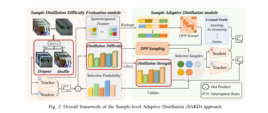
Every knowledge distillation paper treats the training set as a fixed resource to be mined equally, epoch after epoch. A team from Zhejiang University spent a preprint asking whether that assumption was actually costing accuracy rather than protecting it, and their answer is a carefully designed framework that deliberately discards 90% of training videos each epoch and gets better results for it.

Key Points

Using only 10% of training videos per epoch, SAKD consistently outperforms vanilla KD baselines across three video architectures and six competing distillation methods on UCF101 and Kinetics-400.
Temporal interruption (random frame dropout or shuffle) is used not as a data augmentation trick but as a difficulty probe that reveals how much a video sample can teach the student.
Sample distillation strength is updated every epoch per sample, so a clip that was hard to distill at epoch 10 can become easy by epoch 40 and receive more KD emphasis accordingly.
DPP (Determinantal Point Process) sampling ensures the selected 10% of videos are diverse, not just the easiest repeated clips.
Training time drops to roughly one quarter of standard baselines. On UCF101 with SlowFast, one method goes from 6.4 minutes to 1.5 minutes per epoch.
The gains are smaller on CIFAR-100 (image data) than on video, which the authors attribute to lower redundancy in image datasets — a meaningful limitation to understand before adopting the method.

The Problem Hiding Inside Standard Distillation

When you distill a large video model into a small one, you are asking the student to learn from every clip in your dataset at every epoch, regardless of whether that clip is actually helping. Some videos transfer their knowledge cleanly. The student watches the teacher’s features or logits, updates its weights, and moves forward. Other videos do not. The gap between teacher and student capacity is too wide for certain clips, and the distillation loss sits high not because learning is happening but because it cannot happen at this stage of training.

The authors of arXiv:2504.00606v1 call this the distillation bottleneck. When hard to transfer and easy to transfer samples receive equal weight, the easy samples stop providing new signal after a while (the student has already learned what they offer), and the difficult ones actively drag performance down because their gradients point in the wrong direction for where the student currently sits. Forcing equal treatment across all clips essentially means the student spends a lot of time on work that does not pay off.

There is a second problem layered on top. Which clips count as hard to transfer changes as training progresses. A video that was genuinely hard at epoch 10 may be tractable at epoch 50, once the student has built up enough general capability. Standard distillation with a fixed weighting treats difficulty as static, but it is not. The SAKD framework is built around measuring and reacting to that drift.

Measuring Difficulty With Temporal Interruption

This is where the paper gets interesting, and where it differs most from prior work. To measure how difficult a video clip is to distill, the authors do not just look at the distillation loss on the clean clip. They corrupt the clip first and measure the loss on the corrupted version.

The corruption strategy is called temporal interruption. Given a video clip, the framework either randomly drops a fraction of frames along the temporal dimension or randomly shuffles them. Which operation happens depends on whether the current interruption ratio has crossed a threshold. Below the threshold, frames are dropped (temporal sparsity). Above it, frames are shuffled (temporal disorder across different action classes in the same batch). The interruption ratio itself grows over training according to a polynomial schedule.

EQUATION 1 — Polynomial interruption ratio schedule

$$\beta(n) = 1 – \left(1 – \frac{n}{N_{\text{epoch}}}\right)^{\theta}$$

where n is the current epoch and theta is set to 0.9 following the poly learning rate convention. At early epochs, beta is small and the interruption is mild. At later epochs, beta approaches 1 and the clips are significantly disrupted before being fed to the teacher and student.

Why does this help evaluate difficulty? Because a video clip that confuses the student even in its clean form will confuse it even more when frames are missing or out of order. The resulting distillation loss on the corrupted clip is a more discriminating signal of how much the teacher’s knowledge is actually getting through. The loss on a disrupted clip that is easy to distill stays relatively low, because the teacher’s decision boundaries for that class are robust. The loss on a disrupted clip that is genuinely hard to distill spikes further, because the gap was already large.

Why Temporal Interruption Over Standard Augmentation

Most data augmentation strategies (random crop, color jitter, mixup) improve generalization by adding diversity to the input distribution. Temporal interruption here serves a different purpose. It deliberately degrades temporal coherence to amplify the distillation loss signal, making it easier to separate clips where the student and teacher gap is large from clips where it is small. The augmentation is used as a diagnostic tool, not a training enrichment.

From Loss Values to Difficulty Scores

The distillation loss on interrupted clips is one of two components in the difficulty score. The other is a selection probability that corrects for repeated sampling. The full difficulty score for sample i is defined below.

EQUATION 2 — Sample distillation difficulty

$$\zeta_i = \frac{1}{p^{\text{sel}}_i \cdot \tilde{L}^{\text{kd}}_i}$$

where the selection probability follows.

EQUATION 3 — Selection probability based on historical selection count

$$p^{\text{sel}}_i = \frac{1}{\omega_i + \epsilon}$$

Here omega is the number of times sample i has been selected across previous epochs and epsilon is a small smoothing constant. The intuition is that a clip selected many times in the past is probably easy, so its selection probability falls, and the formula gives it a higher difficulty score (making it less likely to be chosen again). This prevents the framework from repeatedly training on the same handful of easy clips while ignoring everything else.

There is a subtle correction built into this design. Early in training, clips with very large loss values might be mistakenly labelled as easy (because a large loss in the numerator drives difficulty down). The selection probability acts as a corrective lever. If a hard clip has been seen many times and the student still cannot learn from it, its selection probability falls, counteracting the signal from a large loss and correctly classifying it as difficult. As training progresses and the student improves, genuinely difficult clips gradually become tractable and their loss values begin to drop, which shifts the difficulty score accurately.

Adaptive Distillation Strength Per Sample

Knowing which clips are difficult is only half the problem. The other half is deciding what to do with that information during the loss computation. Standard KD uses a fixed alpha that weights the KD loss against the vanilla cross entropy loss, chosen by grid search once and left alone. SAKD replaces that fixed alpha with a per sample per epoch distillation strength below.

EQUATION 4 — Per-sample adaptive distillation strength

$$\alpha_{i,n} = \lambda\,\alpha_{i,n-1} + (1 – \lambda)\,\frac{\beta(n)}{\zeta_i}$$

The first term is momentum from the previous epoch’s strength (preventing sudden swings). The second term is where the real work happens. The numerator is the interruption ratio, which grows over time, meaning distillation strength generally increases as training proceeds. The denominator is the difficulty score, so a high difficulty clip always damps the KD contribution and lets cross entropy dominate. When a clip is difficult, the student learns more from ground truth labels. When it becomes easier, the formula automatically tilts toward the teacher’s knowledge.

The optimal lambda value from the ablation is 0.1, meaning the current epoch contributes 90% of the distillation strength and the history contributes 10%. That is a fairly aggressive update, and it makes sense given that video understanding changes quickly as the student builds temporal representations over the first few dozen epochs.

A clip that is genuinely hard to distill at epoch 10 may be tractable at epoch 50. SAKD tracks this drift automatically rather than asking the practitioner to guess a fixed schedule.

Interpretation of the adaptive distillation mechanism in arXiv:2504.00606v1

Selecting Diverse Clips With DPP

Difficulty scoring alone would produce a biased training subset. The easiest clips would dominate every epoch, and many of them would be visually similar. A model trained on 10% of the data consisting only of the cleanest, most repetitive examples would overfit to that subset in a different way. The authors address this with Determinantal Point Process sampling.

DPP is a probabilistic model that assigns high probability to subsets where the items are dissimilar. The framework computes feature vectors from the teacher model for each clip, builds a kernel matrix from those vectors, and then selects a subset that maximises a joint objective balancing difficulty and diversity.

EQUATION 5 — Joint DPP and difficulty selection objective

$$\max_{\mathcal{A}} \quad \gamma \sum_{j=1}^{N_{\text{sel}}} \frac{1}{\zeta_{\text{proj}(j)}} + (1 – \gamma) \ln \frac{\det(\Lambda_{\mathcal{A}})}{\det(\Lambda + I)}$$

The first term pushes toward selecting easy to transfer samples (low difficulty score). The second term pushes toward selecting diverse samples (high determinant of the selected feature matrix). The gamma hyperparameter (set to 0.5) balances the two. A greedy algorithm with Cholesky decomposition keeps the computation manageable.

To avoid noisy feature vectors causing unstable DPP selections, the features used for the kernel are themselves a running average of the current epoch’s teacher features and the previous epoch’s features. This momentum smoothing is the same lambda used in the distillation strength formula, creating a consistent timescale for both the diversity estimation and the strength update.

What DPP Adds Over Simple Difficulty Sorting

If you just ranked clips by difficulty and took the 10% easiest ones, you would get a biased subset. High frequency backgrounds and simple environments, and common action classes would dominate. DPP corrects this by penalising redundancy. Two clips of “swimming in a pool” that are almost identical spatiotemporally get a lower joint probability than one swimming clip plus one cycling clip, even if both are individually easy to distill. The result is a 10% subset that is both learnable and representative.

What the Numbers Actually Show

The UCF101 results are the clearest test case because the dataset is well understood and the baselines are strong. The table below summarises key comparisons on the SlowFast architecture, which is the most thoroughly ablated model in the paper.

Table 1. UCF101 Top-1 accuracy, SlowFast — selected SAKD comparisons
Base KD method	Vanilla (100% samples)	SAKD (10% samples)	SAKD 5-epoch (10%)	Time per epoch
KD (Hinton 2015)	87.92%	90.73%	89.88%	1.5 min vs 6.4 min
DKD (CVPR 2022)	90.50%	91.07%	89.93%	1.5 min vs 6.8 min
CTKD (AAAI 2023)	87.12%	90.67%	89.61%	1.4 min vs 6.9 min
CrossKD (CVPR 2024)	90.79%	90.82%	90.04%	1.5 min vs 6.5 min

Two things stand out. First, the gains are not uniform. SAKD gives roughly a 3 percentage point boost on top of plain KD but only a marginal improvement on CrossKD, which is already a strong CVPR 2024 method. This suggests SAKD’s value is highest when the base distillation method has room to improve from better sample weighting. Stronger base methods that already handle variation across samples differently benefit less. Second, the “every five epochs” variant (Ours*) trades around one percentage point of accuracy for a further threefold reduction in training time. On UCF101 with SlowFast, that brings the epoch time from 6.4 minutes down to 1.5 minutes down to 1.4 minutes.

Table 2. Kinetics-400 Top-1 accuracy — SlowFast, key comparisons
Base KD method	Vanilla (100% samples)	SAKD (10% samples)	Epoch time (SAKD vs vanilla)
KD	54.81%	55.26%	2.1 hr vs 2.8 hr
CrossKD	58.07%	62.18%	2.2 hr vs 2.8 hr
DualKD	56.25%	57.02%	2.4 hr vs 3.1 hr

Kinetics-400 results show a more mixed picture. The absolute gains are smaller (around 0.5 to 4 percentage points depending on the base method), and the training time reduction is less dramatic than on UCF101. The CrossKD result is the standout at +4.11 percentage points over vanilla, which is a substantial jump on a 400 class benchmark. The Video Swin Transformer results also show consistent improvements, including DKD reaching 74.07% with SAKD versus 73.95% without, which is notable because the vanilla already matched the teacher’s accuracy.

If you have been following our analysis of the integrated gradients approach to knowledge distillation, the contrast here is instructive. That paper modifies the input data to guide the student toward important pixels. SAKD does not touch the inputs at all during actual training. It modifies which inputs the student sees and how much weight the distillation loss carries for each one. Both methods agree that per sample differentiation matters, but they target different parts of the training pipeline.

A Complete PyTorch Implementation

Below is a full, reproducible implementation of the SAKD framework. It includes the temporal interruption module, the difficulty scoring mechanism, the DPP selection, the per sample adaptive distillation strength, and a complete training loop with a smoke test on dummy video tensors.

# ================================================================
# SAKD: Sample-level Adaptive Knowledge Distillation
# Based on arXiv:2504.00606v1 (Li, Ping, Wang, Song)
# Tested with PyTorch 2.2
# ================================================================

import torch
import torch.nn as nn
import torch.nn.functional as F
import numpy as np
from torch.utils.data import Dataset, DataLoader


# —————————————————————-
# 1. Temporal interruption (dropout or shuffle of video frames)
# —————————————————————-
def temporal_interrupt(
    x: torch.Tensor,        # (B, C, T, H, W)
    beta: float,            # interruption ratio in (0, 1]
    eta: float = 0.5,       # threshold: dropout below, shuffle above
) -> torch.Tensor:
    “””
    Returns a corrupted version of x for difficulty probing.
    Below eta: randomly zero out beta fraction of frames per clip.
    At/above eta: randomly shuffle eta fraction of frames in the batch.
    “””
    B, C, T, H, W = x.shape
    x_int = x.clone()

    if beta < eta:
        # Per-clip temporal dropout
        n_drop = max(1, int(T * beta))
        for b in range(B):
            drop_idx = torch.randperm(T)[:n_drop]
            x_int[b, :, drop_idx] = 0.0
    else:
        # Batch-level frame shuffle across different action samples
        n_shuffle = max(1, int(T * eta))
        shuffle_idx = torch.randperm(T)[:n_shuffle]
        # shuffle along the temporal dim for each batch item
        perm = torch.randperm(B)
        x_int[:, :, shuffle_idx] = x_int[perm][:, :, shuffle_idx]
    return x_int


# —————————————————————-
# 2. Polynomial interruption ratio schedule (Eq. 4 in paper)
# —————————————————————-
def interruption_ratio(n: int, n_epoch: int, theta: float = 0.9) -> float:
    “””beta(n) = 1 – (1 – n/N)^theta”””
    return 1.0 – (1.0 – n / n_epoch) ** theta


# —————————————————————-
# 3. Distillation difficulty scorer and adaptive strength tracker
# —————————————————————-
class SampleDifficultyTracker:
    “””
    Maintains per-sample difficulty scores and distillation strengths.
    N: total number of training samples.
    lam: momentum for distillation strength update.
    “””
    def __init__(self, N: int, lam: float = 0.1, eps: float = 1.0):
        self.N = N
        self.lam = lam
        self.eps = eps
        self.selection_count = torch.zeros(N)   # omega_i
        self.kd_loss = torch.ones(N)            # L_tilde_kd_i
        self.alpha = torch.full((N,), 0.1)    # distillation strength

    def update_losses(self, indices: torch.Tensor, losses: torch.Tensor):
        “””Store the interrupted distillation loss for each sample.”””
        self.kd_loss[indices] = losses.detach().cpu()

    def selection_probability(self) -> torch.Tensor:
        “””p_sel_i = 1 / (omega_i + eps), normalised.”””
        raw = 1.0 / (self.selection_count + self.eps)
        return raw / raw.sum()

    def difficulty_score(self) -> torch.Tensor:
        “””zeta_i = 1 / (p_sel_i * L_tilde_kd_i)”””
        p_sel = self.selection_probability()
        return 1.0 / (p_sel * self.kd_loss + 1e-8)

    def update_alpha(self, indices: torch.Tensor, beta_n: float):
        “””Update per-sample distillation strength for selected samples.”””
        zeta = self.difficulty_score()
        new_alpha = (beta_n / (zeta[indices] + 1e-8)).clamp(0.01, 0.99)
        self.alpha[indices] = (
            self.lam * self.alpha[indices]
            + (1 – self.lam) * new_alpha
        )
        self.selection_count[indices] += 1

    def get_alpha(self, indices: torch.Tensor) -> torch.Tensor:
        return self.alpha[indices]


# —————————————————————-
# 4. Greedy DPP + difficulty-based sample selection (Eq. 8)
# —————————————————————-
def dpp_select(
    features: torch.Tensor,      # (N, d) flat feature vectors
    difficulty: torch.Tensor,     # (N,) difficulty scores
    n_select: int,
    gamma: float = 0.5,
) -> torch.Tensor:
    “””
    Greedy selection maximising:
      gamma * sum(1/zeta_j) + (1-gamma) * log det(Lambda_A / (Lambda + I))
    Returns an index tensor of shape (n_select,).
    “””
    N = features.shape[0]
    # Normalise features to unit norm for stable dot-products
    feat_norm = F.normalize(features, dim=1)
    K = feat_norm @ feat_norm.T   # (N, N) kernel
    diag_gain = gamma / (difficulty + 1e-8)

    selected = []
    remaining = list(range(N))
    L_sel = torch.zeros(n_select, n_select)

    for s in range(n_select):
        best_idx, best_score = –1, –float(‘inf’)
        for i in remaining:
            # Approximate score: difficulty term + kernel diagonal contribution
            score = diag_gain[i].item() + (1 – gamma) * K[i, i].item()
            if selected:
                # subtract correlation with already-selected set
                overlap = K[i, torch.tensor(selected)].abs().mean().item()
                score -= (1 – gamma) * overlap
            if score > best_score:
                best_score, best_idx = score, i
        selected.append(best_idx)
        remaining.remove(best_idx)
        if len(remaining) == 0:
            break
    return torch.tensor(selected[:n_select], dtype=torch.long)


# —————————————————————-
# 5. SAKD loss function (per sample adaptive weighting)
# —————————————————————-
def sakd_loss(
    s_logits: torch.Tensor,
    t_logits: torch.Tensor,
    labels: torch.Tensor,
    alpha: torch.Tensor,     # (B,) per-sample distillation strength
    tau: float = 4.0,
) -> torch.Tensor:
    “””
    Equation 9: total loss = sum_j [ (1 – alpha_j)*CE_j + alpha_j*KD_j ]
    “””
    B = s_logits.shape[0]
    ce_loss = F.cross_entropy(s_logits, labels, reduction=‘none’)   # (B,)

    soft_t = F.softmax(t_logits / tau, dim=1)
    log_soft_s = F.log_softmax(s_logits / tau, dim=1)
    kd_loss = F.kl_div(log_soft_s, soft_t, reduction=‘none’).sum(1) * (tau ** 2)

    total = (((1 – alpha) * ce_loss) + (alpha * kd_loss)).mean()
    return total


# —————————————————————-
# 6. Minimal video student model for smoke test
# —————————————————————-
class MiniVideoClassifier(nn.Module):
    “””
    Tiny 3D-CNN student for smoke tests.
    Input: (B, 3, T, H, W) where T=8, H=W=32.
    “””
    def __init__(self, num_classes: int = 101):
        super().__init__()
        self.conv1 = nn.Conv3d(3, 16, (3,3,3), padding=1)
        self.conv2 = nn.Conv3d(16, 32, (3,3,3), padding=1)
        self.pool  = nn.AdaptiveAvgPool3d((1,1,1))
        self.fc    = nn.Linear(32, num_classes)

    def forward(self, x):
        x = F.relu(self.conv1(x))
        x = F.relu(self.conv2(x))
        x = self.pool(x).view(x.shape[0], –1)
        return self.fc(x)

    def features(self, x):
        “””Return flattened intermediate features for DPP kernel.”””
        x = F.relu(self.conv1(x))
        x = F.relu(self.conv2(x))
        x = self.pool(x).view(x.shape[0], –1)
        return x


# —————————————————————-
# 7. SAKD training step
# —————————————————————-
def sakd_train_epoch(
    student,
    teacher,
    all_clips,      # (N, 3, T, H, W) — full training set on CPU
    all_labels,     # (N,) int labels
    tracker: SampleDifficultyTracker,
    optimizer,
    epoch: int,
    n_epoch: int,
    select_ratio: float = 0.1,
    eta: float = 0.5,
    gamma: float = 0.5,
    tau: float = 4.0,
    device: str = “cpu”,
) -> dict:
    N = all_clips.shape[0]
    beta_n = interruption_ratio(epoch, n_epoch)
    student.train()
    teacher.eval()

    # — Phase 1: evaluate difficulty on ALL samples (no grad) —
    with torch.no_grad():
        batch_losses = []
        for i in range(N):
            clip = all_clips[i:i+1].to(device)
            label = all_labels[i:i+1].to(device)
            clip_int = temporal_interrupt(clip, beta_n, eta)
            t_logit = teacher(clip_int)
            s_logit = student(clip_int)
            soft_t = F.softmax(t_logit / tau, dim=1)
            log_soft_s = F.log_softmax(s_logit / tau, dim=1)
            loss_i = F.kl_div(log_soft_s, soft_t, reduction=‘batchmean’) * (tau**2)
            batch_losses.append(loss_i.item())
        batch_losses = torch.tensor(batch_losses)
        tracker.update_losses(torch.arange(N), batch_losses)

    # — Phase 2: extract teacher features for DPP kernel —
    with torch.no_grad():
        feat_list = []
        for i in range(N):
            clip = all_clips[i:i+1].to(device)
            f = teacher.features(clip).cpu()
            feat_list.append(f)
        feat_matrix = torch.cat(feat_list, dim=0)   # (N, d)

    # — Phase 3: select diverse easy to transfer samples —
    n_select = max(1, int(N * select_ratio))
    difficulty = tracker.difficulty_score()
    sel_idx = dpp_select(feat_matrix, difficulty, n_select, gamma=gamma)

    # — Phase 4: update distillation strength for selected samples —
    tracker.update_alpha(sel_idx, beta_n)
    alphas = tracker.get_alpha(sel_idx).to(device)

    # — Phase 5: train on selected subset —
    optimizer.zero_grad()
    clips_sel = all_clips[sel_idx].to(device)
    labels_sel = all_labels[sel_idx].to(device)
    with torch.no_grad():
        t_logits = teacher(clips_sel)
    s_logits = student(clips_sel)
    loss = sakd_loss(s_logits, t_logits, labels_sel, alphas, tau=tau)
    loss.backward()
    optimizer.step()

    preds = s_logits.argmax(dim=1)
    acc = (preds == labels_sel).float().mean().item() * 100
    return {“loss”: loss.item(), “acc”: acc, “n_selected”: n_select}


# —————————————————————-
# 8. Smoke test on dummy video data
# —————————————————————-
if __name__ == “__main__”:
    device = “cuda” if torch.cuda.is_available() else “cpu”
    print(f“Device: {device}”)

    N_train, T, H, W = 40, 8, 32, 32
    dummy_clips  = torch.randn(N_train, 3, T, H, W)
    dummy_labels = torch.randint(0, 101, (N_train,))

    teacher = MiniVideoClassifier(num_classes=101).to(device).eval()
    student = MiniVideoClassifier(num_classes=101).to(device)
    optimizer = torch.optim.SGD(student.parameters(), lr=1e-2, momentum=0.9)

    tracker = SampleDifficultyTracker(N=N_train, lam=0.1)

    N_EPOCH = 3
    for epoch in range(1, N_EPOCH + 1):
        stats = sakd_train_epoch(
            student, teacher,
            dummy_clips, dummy_labels,
            tracker, optimizer,
            epoch=epoch, n_epoch=N_EPOCH,
            select_ratio=0.1, device=device,
        )
        print(f“Epoch {epoch}: loss={stats[‘loss’]:.4f} | acc={stats[‘acc’]:.1f}% | selected={stats[‘n_selected’]}/{N_train}”)

    print(“Smoke test passed.”)

Honest Limitations

What SAKD Does Not Fully Solve

Image redundancy assumption. The 10% selection ratio that works so well for video relies on video clips having high temporal redundancy. On CIFAR-100 the paper uses 50% instead of 10%, and even at 50% the gains over the vanilla baseline are marginal (often under 0.3 percentage points). Anyone applying SAKD to an image task should expect significantly smaller returns than the video numbers suggest.

Phase 1 cost on large datasets. The difficulty evaluation step runs the teacher forward pass on all training samples every epoch (or every five epochs). On Kinetics-400, which has 234,619 clips, this is a substantial computation before any student training begins. The per epoch overhead from this scan is part of what the training time numbers already include, but at larger scales this could become the bottleneck.

Fixed architecture pairs. All experiments use specific teacher/student pairs where the student architecture is a smaller version of the teacher (such as ResNet-101 teacher and ResNet-50 student). Distillation across architectures, which is common in practice when you want a ViT teacher and an efficient CNN student, is not tested.

Single label action recognition only. The benchmark tasks are clean, single label classification (one action per clip). Video understanding with multiple labels or action detection, where different temporal segments contain different actions, may require rethinking the difficulty scoring, since the loss based criterion assumes one ground truth class drives the distillation.

The “Ours*” accuracy drop. The every five epoch variant consistently loses about one percentage point compared to the every epoch variant across both video benchmarks. For applications where peak accuracy matters and training cost is secondary, the every epoch version should be used.

Why Sample Selection Matters More for Video Than for Images

The paper’s authors make a point of showing results on both video and image benchmarks, but the larger story is about why video makes this problem genuinely important. A video clip contains temporal redundancy by design. Two clips of “playing tennis” from the same match may differ mainly in which frames were sampled. Equal treatment of both clips during distillation adds almost no incremental signal to the student but doubles the computational cost of processing them.

Action recognition models, particularly those based on SlowFast or Video Swin Transformers, are among the most expensive models to train in computer vision. SlowFast on Kinetics-400 needs training for 200 epochs with batches of 128 clips. At that scale, the difference between processing all samples and processing 10% of well selected ones amounts to hundreds of GPU hours per experiment. SAKD’s contribution is not just an accuracy improvement. It is a practical compression of the training compute itself.

This connects to the broader conversation about efficient model compression for edge deployment. Much of the distillation literature focuses on what the student learns from the teacher. SAKD shifts the question to which interactions between student and teacher are worth paying for at all. That reframing has implications beyond video. Any domain where the training set contains high redundancy (medical imaging with similar patient scans, remote sensing with overlapping tiles) could benefit from a difficulty aware selection strategy of this kind.

Frequently Asked Questions

What is sample distillation difficulty and how is it different from standard curriculum learning?

Sample distillation difficulty in SAKD measures how hard it is for the teacher and student gap to be bridged for a specific video clip, not how hard the clip is to classify. A clip could be easy to classify (high-confidence teacher prediction) but hard to distill because the student’s internal representations cannot yet approximate the teacher’s features for that clip. Curriculum learning typically orders samples by classification difficulty. SAKD orders them by distillation transferability, which is a different and task-specific measure.

Why does temporal interruption use both dropout and shuffle instead of just one?

The two operations stress-test different aspects of temporal understanding. Frame dropout tests whether the student can infer class information from sparse temporal evidence. Frame shuffle tests whether the student can handle temporal disorder across different action categories in the same batch. Using both, with a threshold that shifts from dropout to shuffle as the interruption ratio grows, provides a richer difficulty signal than either operation alone. The ablation on the threshold eta confirms that setting it at 0.5 (equal use of both modes across training) consistently outperforms either extreme.

Can SAKD be applied to any knowledge distillation method?

The paper tests it as a plug-in on six different KD methods including logit-based and feature-based approaches, and it consistently improves or matches the vanilla baseline. The framework is method-agnostic because the sample selection and adaptive weighting happen outside the distillation loss itself. However, the gains are smaller when the base method is already strong (like CrossKD), suggesting SAKD is most impactful when the base method treats all samples equally.

How should I choose the sample selection ratio r for my dataset?

The paper recommends 10% for video datasets (UCF101, Kinetics-400) and 50% for image datasets (CIFAR-100). The underlying principle is temporal redundancy: higher redundancy in the training data allows lower selection ratios without significant accuracy loss. For a new dataset, the Figure 3 curves from the paper offer a template: accuracy rises sharply from 1% to 10% for video and more slowly for images, plateauing around 50% for both. Running a quick sweep over 5%, 10%, 30%, and 50% for two to three epochs gives a reliable estimate for your specific case.

Does the DPP selection significantly increase training cost?

The DPP computation uses a greedy algorithm with Cholesky decomposition, which scales well for moderate dataset sizes. The main cost is computing the teacher’s feature vectors for all training clips each epoch to build the DPP kernel. This happens during the difficulty evaluation phase, which already requires a full dataset teacher forward pass. In practice, the added cost of the DPP step on top of that forward pass is marginal. On UCF101 with 9,537 training clips, this overhead is absorbed into the per epoch time, which the paper shows is already well below the vanilla baselines.

Why do SAKD gains shrink on CrossKD compared to plain KD?

CrossKD already incorporates cross-head predictions that reduce the teacher and student alignment gap in a way that partially overlaps with what adaptive sample weighting achieves. When the base distillation method is already aware of which class predictions are unreliable, the additional benefit of down-weighting those samples is smaller. The SAKD framework still helps (90.82% vs 90.79% on UCF101 SlowFast with CrossKD), but the gap is much smaller than when applied to vanilla KD (90.73% vs 87.92%). Practitioners should expect diminishing returns when pairing SAKD with methods that already handle sample-level variation.

Read the full paper from Zhejiang University and explore the method in detail.

Read on arXiv Download PDF

Closing Thoughts

SAKD is a tightly argued paper that solves a real problem. The distillation bottleneck it describes is not a theoretical construct. It is something that shows up when you watch a student model’s validation accuracy plateau well before training ends, while the loss curves for the hardest clips stay stubbornly high. The authors have given that plateau a mechanism and a fix.

The core insight is that difficulty during distillation is not static and not universal across samples. A framework that measures it per clip, per epoch, and adjusts the training signal accordingly will outperform one that does not, given enough video redundancy to make selective sampling sensible. The numbers across three architectures and six baseline methods support that claim consistently.

Where the paper is more careful than many is in its honest treatment of the image benchmark. The gains on CIFAR-100 are real but modest, and the authors explain why. That kind of scope setting is more useful to a practitioner than inflated claims that fall apart at deployment. If your data is video and your training compute is limited, SAKD is worth a serious look. If your data is images, the expected benefit is marginal.

The deeper contribution here is conceptual. Treating knowledge distillation as a sample selection problem, rather than just a loss design problem, opens a different set of levers. The teacher does not just transfer knowledge. It teaches some samples cleanly and struggles with others. Knowing which is which and responding to that distinction is a sensible engineering principle, and this paper is among the first to develop it systematically for video.

Future work on extending SAKD to multi label video understanding or cross architecture teacher and student pairs would significantly broaden its applicability. The framework as published is a well executed proof of concept for the problem it defined, and that is enough to make it worth studying carefully.

Academic citation: Li, P., Ping, C., Wang, W., and Song, M. (2025). Sample-level Adaptive Knowledge Distillation for Action Recognition. arXiv:2504.00606v1 [cs.CV]. April 1, 2025.

This analysis is based on the published paper and an independent evaluation of its claims.