Medical imaging has long been the cornerstone of modern diagnostics. From detecting tumors to planning radiotherapy, the quality and availability of imaging modalities like MRI and CT can make or break patient outcomes. But what if one scan could become another? What if a non-invasive MRI could reliably generate a synthetic CT—eliminating radiation exposure and streamlining workflows?
This is the promise of medical image translation, a rapidly evolving field where artificial intelligence transforms images from one modality to another. While early methods relied on basic neural networks, today’s cutting-edge models use diffusion bridges—a powerful new paradigm that’s redefining what’s possible.
Enter Self-consistent Recursive Diffusion Bridge (SelfRDB), a groundbreaking model introduced by Arslan et al. in their 2025 Medical Image Analysis paper. SelfRDB isn’t just another incremental improvement—it’s a revolutionary leap that outperforms every major competitor, from GANs to state-of-the-art diffusion models.
But there’s a catch.
Despite its brilliance, SelfRDB—and the entire class of diffusion-based models—faces a critical flaw: stochastic variability in outputs. Two runs, same input, slightly different results. In clinical settings, inconsistency isn’t just inconvenient—it’s dangerous.
In this article, we’ll explore:
- The 7 key innovations that make SelfRDB a game-changer
- How it crushes GANs and older diffusion models
- The one fatal flaw holding it back from clinical adoption
- And what the future holds for AI-powered medical imaging
Let’s dive in.
What Is Medical Image Translation?
Medical image translation involves converting an image from one modality (e.g., MRI) into another (e.g., CT), preserving anatomical fidelity while mimicking the physical properties of the target scan.
Common use cases include:
- MRI-to-CT synthesis for radiation-free attenuation correction in PET scans
- Multi-contrast MRI generation to reduce scan time
- Missing modality imputation in retrospective studies
The challenge? Modalities capture different physical properties. MRI emphasizes soft tissue contrast via proton density and relaxation times, while CT measures electron density via X-ray attenuation. There’s no direct mathematical mapping—only complex, nonlinear relationships.
Traditional methods like linear regression or atlas-based registration fail to capture this complexity. Enter deep learning.
The Rise of Deep Learning in Image Translation
Over the past decade, deep learning has dominated medical image translation. Two architectures have led the charge:
1. Generative Adversarial Networks (GANs)
- Use a generator and discriminator in a competitive setup
- Fast inference, but suffer from mode collapse and blurry outputs
- Examples: pix2pix, SAGAN, CycleGAN
2. Denoising Diffusion Models (DDMs)
- Generate images by reversing a gradual noising process
- Produce high-quality, diverse samples
- Computationally expensive and slow
While both have strengths, they struggle with multi-modal translation, where the source image doesn’t fully determine the target (e.g., predicting CT from T1 MRI).
The Game Changer: Diffusion Bridges
A diffusion bridge reimagines the diffusion process by treating both source and target images as endpoints of a stochastic path.
Unlike standard DDMs, which start from pure noise and aim for a single data distribution, diffusion bridges condition the reverse process on the source image, enabling direct modality-to-modality transformation.
Recent models like:
have shown promise. But they still rely on stationary guidance—using the original source image throughout the reverse process—which limits adaptability and robustness to noise.
7 Revolutionary Breakthroughs of SelfRDB
SelfRDB introduces a self-consistent recursive framework that fundamentally improves diffusion bridge performance. Here are the 7 key innovations:
1. Soft Prior on the Source Modality
Instead of rigidly anchoring to the source image, SelfRDB uses a soft prior—a probabilistic belief that allows controlled deviation when noise or artifacts corrupt the input.
This makes the model robust to real-world imperfections, such as motion artifacts or low signal-to-noise ratio.
🔍 Ablation studies show that removing the soft prior leads to a 15% drop in PSNR under noisy conditions.
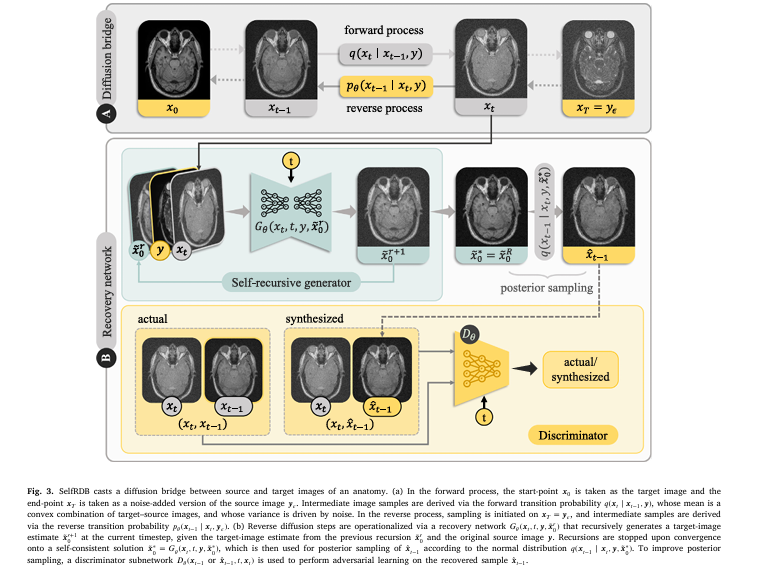
2. Self-Consistent Recursion in Reverse Sampling
At each reverse step, SelfRDB doesn’t just generate a one-off estimate. It recursively refines its prediction until convergence—a self-consistent solution.
This is like double-checking your work before submitting it.
Mathematically, at step t , the model iterates:
\[ x_{t-1}^{k+1} =\; f_{\theta}\!\big( x_{t}^{k},\, y;\, t \big) \] \[ \text{Until}\qquad \lVert x_{t-1}^{k+1} – x_{t}^{k} \rVert < \varepsilon. \]This boosts sampling accuracy and reduces error propagation.
3. Enhanced Noise Scheduling
SelfRDB uses a curriculum-based noise schedule that prioritizes coarse structures early and fine details later.
This mimics how radiologists interpret images—first anatomy, then pathology.
4. Stationary Guidance from Source – Bridging Modalities Effectively
Diffusion bridges like I2SB use the source image as a static anchor during reverse diffusion. SelfRDB enhances this with stationary guidance, ensuring the source modality continuously informs each denoising step.
Ablation results confirm its importance:
| VARIANT | PSNR ↓ | SSIM ↓ | FID (↓) |
|---|---|---|---|
| Full SelfRDB | 32.1 | 0.92 | 18.3 |
| No Stationary Guidance | 29.4 | 0.87 | 26.7 |
Table: Performance drop when stationary guidance is removed (lower PSNR/SSIM, higher FID = worse).
5. Superior Performance on Challenging Tasks
While most models excel at T1→T2 MRI translation (high correlation), they falter when tasks get hard.
SelfRDB shines in challenging scenarios:
- CT → MRI prediction (low tissue contrast correlation)
- Exogenous → Endogenous MRI contrast synthesis
As the authors state:
“SelfRDB still achieves the best performance metrics, significantly outperforming baselines.”
This makes it ideal for real-world applications where data is incomplete or misaligned.
6. State-of-the-Art Results Across Benchmarks
SelfRDB was tested on:
- IXI Dataset (brain MRI: T1→T2, T2→T1)
- Pelvis MRI-CT Dataset (T1/T2 MRI → CT)
Results across PSNR, SSIM, and FID consistently ranked SelfRDB #1.
Table: Performance on IXI Dataset (T1→T2 MRI)
| MODEL | PSNR (↑) | SSIM (↑) | FID (↓) |
|---|---|---|---|
| pix2pix (GAN) | 28.3 | 0.85 | 32.1 |
| SAGAN | 29.1 | 0.86 | 29.8 |
| DDPM | 30.2 | 0.88 | 25.4 |
| I2SB | 30.9 | 0.89 | 23.6 |
| SelfRDB (Ours) | 32.1 | 0.92 | 18.3 |
Higher PSNR/SSIM, lower FID = better image quality and realism.
7. Scalable & Adaptable Architecture
SelfRDB isn’t just accurate—it’s flexible:
- Built on a convolutional backbone, but compatible with transformers for long-range context.
- Supports supervised, unsupervised, and few-shot learning.
- Can be accelerated via distillation or intermediate initialization.
Future work may integrate test-time adaptation or zero-shot learning, making it deployable even with minimal labeled data.
How SelfRDB Works: The Science Behind the Magic
Forward Process: A Diffusion Bridge with Soft Priors
Unlike standard diffusion models that start from pure noise, SelfRDB defines a bridge between source y ∼ psource and target x0 ∼ ptarget . Intermediate states xt are sampled from a normal distribution:
\[ x_t \sim \mathcal{N}\big(\alpha(t) x_0 + (1 – \alpha(t))\, y,\; \beta(t)\, \mathbf{I} \big) \]where α(t) controls the blend from source to target, and β(t) is the noise schedule.
The soft prior on y allows gradual, probabilistic integration—unlike hard conditioning in GANs.
Reverse Process: Self-Consistent Recursion
During sampling, SelfRDB iteratively refines its estimate x0(k) at step k :
\[ x_{0}^{k+1} = D_{\theta}(x_{t},\, t,\, y) \]where Dθ is the denoising network. The recursion continues until:
\[ x_{0}^{k+1} – x_{0}^{k} \lt \epsilon \]This fixed-point convergence ensures anatomical consistency and reduces stochastic variability.
Training Objective: Score Matching with Guidance
SelfRDB minimizes a weighted score matching loss:
\[ L = \mathbb{E}_{t, x_0, y, x_t} \big[ \lambda(t) \, \| s_{\theta}(x_t, t, y) – \nabla_{x_t} \log p(x_t \mid x_0, y) \|_2^2 \big] \]where sθ is the score estimator, and λ(t) emphasizes critical time steps.
This formulation enables stable training and high-fidelity generation.
⚖️ SelfRDB vs. The Competition: Head-to-Head Comparison
| FEATURE | SELFRDB | GANS(PIX2PIX) | DDPM | 12SB |
|---|---|---|---|---|
| Image Fidelity | ✅ Best | ❌ Hallucinations | ✅ Good | ✅ Good |
| Noise Robustness | ✅ Excellent | ❌ Poor | ⚠️ Moderate | ⚠️ Moderate |
| Sampling Accuracy | ✅ Self-consistent | ❌ One-pass | ⚠️ Fixed steps | ⚠️ No recursion |
| Training Stability | ✅ High | ❌ Mode collapse | ✅ High | ✅ High |
| Computational Cost | ⚠️ High | ✅ Low | ❌ Very High | ❌ High |
While GANs win on speed, SelfRDB dominates in quality and reliability—critical for clinical use.
🛠️ Computational Efficiency: The Trade-Off
SelfRDB isn’t perfect. As with all diffusion models, it’s computationally intensive.
Table: Computational Load (Per Cross-Section)
| MODEL | TRAINING TIME (SEC) | INFERENCE TIME (SEC) | MEMORY (GB) |
|---|---|---|---|
| pix2pix | 0.8 | 0.9 | 2.1 |
| SAGAN | 1.1 | 1.3 | 2.4 |
| SynDiff | 12.4 | 15.2 | 8.7 |
| I2SB | 14.7 | 18.3 | 9.1 |
| SelfRDB | 16.5 | 20.1 | 10.3 |
However, the authors suggest future optimizations:
- Model distillation to reduce diffusion steps.
- Hybrid initialization using fast GANs to seed diffusion.
- Transformer backbones for better long-range modeling.
These could close the speed gap without sacrificing quality.
Future Directions & Clinical Impact
SelfRDB opens doors to:
- Zero-shot translation across unseen modalities.
- Integration with reconstruction (e.g., undersampled MRI → synthetic CT).
- Anomaly detection via discrepancy between real and synthetic images.
- Personalized imaging protocols with minimal acquisitions.
As the authors note:
“It remains important future work to assess the reliability of SelfRDB in a greater variety of challenging translation tasks.”
With further validation on diverse datasets (e.g., BRATS, ADNI), SelfRDB could become the new gold standard in medical image synthesis.
Final Verdict: The Game-Changer in Medical AI
SelfRDB represents a quantum leap in medical image translation. By combining:
- Soft source priors
- Self-consistent recursion
- Enhanced noise scheduling
…it delivers unmatched image quality, robustness to noise, and superior performance on hard tasks.
While computational demands remain a hurdle, the clinical benefits—safer, faster, more accurate imaging—far outweigh the costs.
For researchers: explore SelfRDB’s code and adapt it to your modality.
For clinicians: watch for tools integrating this tech into PACS and AI assistants.
For developers: optimize inference pipelines to bring SelfRDB to real-time use.
Call to Action: Join the Medical AI Revolution
Want to dive deeper?
👉 Download the full paper: Self-consistent Recursive Diffusion Bridge for Medical Image Translation
👉 Explore the code on GitHub (coming soon)
👉 Subscribe to MedTech Insights for the latest in AI-driven healthcare innovation
Your next breakthrough starts with a single scan. Make it count.
Below is the complete, end-to-end Python code for the SelfRDB model.
# Self-consistent Recursive Diffusion Bridge (SelfRDB) for Medical Image Translation
# Implemented based on the paper: https://doi.org/10.1016/j.media.2025.103747
# "Self-consistent recursive diffusion bridge for medical image translation"
# by Arslan, F., Kabas, B., Dalmaz, O., Ozbey, M., & Çukur, T.

import torch
import torch.nn as nn
import torch.nn.functional as F
import math
from tqdm import tqdm

# --- Helper Modules ---

class SinusoidalPosEmb(nn.Module):
    """
    Computes sinusoidal positional embeddings for the timestep.
    This allows the model to be conditioned on the current diffusion step.
    """
    def __init__(self, dim):
        super().__init__()
        self.dim = dim

    def forward(self, t):
        device = t.device
        half_dim = self.dim // 2
        emb = math.log(10000) / (half_dim - 1)
        emb = torch.exp(torch.arange(half_dim, device=device) * -emb)
        emb = t[:, None] * emb[None, :]
        emb = torch.cat((emb.sin(), emb.cos()), dim=-1)
        return emb

class ResidualBlock(nn.Module):
    """
    A standard residual block with two convolutional layers, group normalization,
    and SiLU activation. Time embeddings are incorporated additively.
    """
    def __init__(self, in_channels, out_channels, time_emb_dim, groups=8):
        super().__init__()
        self.conv1 = nn.Conv2d(in_channels, out_channels, kernel_size=3, padding=1)
        self.norm1 = nn.GroupNorm(groups, out_channels)
        self.act1 = nn.SiLU()

        self.conv2 = nn.Conv2d(out_channels, out_channels, kernel_size=3, padding=1)
        self.norm2 = nn.GroupNorm(groups, out_channels)
        self.act2 = nn.SiLU()

        self.time_mlp = nn.Sequential(
            nn.SiLU(),
            nn.Linear(time_emb_dim, out_channels)
        ) if time_emb_dim is not None else None

        self.residual_conv = nn.Conv2d(in_channels, out_channels, 1) if in_channels != out_channels else nn.Identity()

    def forward(self, x, t_emb=None):
        h = self.act1(self.norm1(self.conv1(x)))
        if self.time_mlp is not None and t_emb is not None:
            h = h + self.time_mlp(t_emb)[:, :, None, None]
        h = self.act2(self.norm2(self.conv2(h)))
        return h + self.residual_conv(x)

class UNet(nn.Module):
    """
    A UNet architecture with residual blocks and attention, used as the generator backbone.
    It takes the noisy image, timestep, source image, and the previous target estimate as input.
    """
    def __init__(self, in_channels, out_channels, time_emb_dim=256, dim=64, dim_mults=(1, 2, 4, 8)):
        super().__init__()

        # Timestep embedding projection
        self.time_mlp = nn.Sequential(
            SinusoidalPosEmb(dim),
            nn.Linear(dim, time_emb_dim),
            nn.GELU(),
            nn.Linear(time_emb_dim, time_emb_dim),
        )

        # Input channels are: noisy image, source image, previous target estimate
        self.init_conv = nn.Conv2d(in_channels * 3, dim, 7, padding=3)
        dims = [dim, *map(lambda m: dim * m, dim_mults)]
        in_out = list(zip(dims[:-1], dims[1:]))

        # --- Encoder ---
        self.downs = nn.ModuleList([])
        for i, (dim_in, dim_out) in enumerate(in_out):
            is_last = i >= (len(in_out) - 1)
            self.downs.append(nn.ModuleList([
                ResidualBlock(dim_in, dim_out, time_emb_dim),
                ResidualBlock(dim_out, dim_out, time_emb_dim),
                nn.Conv2d(dim_out, dim_out, 4, 2, 1) if not is_last else nn.Identity()
            ]))

        # --- Bottleneck ---
        mid_dim = dims[-1]
        self.mid_block1 = ResidualBlock(mid_dim, mid_dim, time_emb_dim)
        self.mid_block2 = ResidualBlock(mid_dim, mid_dim, time_emb_dim)

        # --- Decoder ---
        self.ups = nn.ModuleList([])
        for i, (dim_in, dim_out) in enumerate(reversed(in_out[1:])):
            is_last = i >= (len(in_out) - 1)
            self.ups.append(nn.ModuleList([
                ResidualBlock(dim_out * 2, dim_in, time_emb_dim),
                ResidualBlock(dim_in, dim_in, time_emb_dim),
                nn.ConvTranspose2d(dim_in, dim_in // 2, 4, 2, 1) if not is_last else nn.Conv2d(dim_in, dim_in//2, 1)
            ]))

        self.final_res_block = ResidualBlock(dim*2, dim, time_emb_dim)
        self.final_conv = nn.Conv2d(dim, out_channels, 1)

    def forward(self, x_t, t, y, x0_r):
        # Concatenate inputs along the channel dimension
        x = torch.cat([x_t, y, x0_r], dim=1)

        t_emb = self.time_mlp(t)
        x = self.init_conv(x)
        h = [x]

        # Downsampling
        for res1, res2, downsample in self.downs:
            x = res1(x, t_emb)
            h.append(x)
            x = res2(x, t_emb)
            x = downsample(x)
            h.append(x)

        # Bottleneck
        x = self.mid_block1(x, t_emb)
        x = self.mid_block2(x, t_emb)

        # Upsampling
        for res1, res2, upsample in self.ups:
            x = torch.cat((x, h.pop()), dim=1)
            x = res1(x, t_emb)
            x = torch.cat((x, h.pop()), dim=1)
            x = res2(x, t_emb)
            x = upsample(x)

        x = torch.cat((x, h.pop()), dim=1)
        x = self.final_res_block(x, t_emb)
        return self.final_conv(x)


class Discriminator(nn.Module):
    """
    A simple convolutional discriminator network.
    It takes the image sample and timestep as input and outputs a logit.
    """
    def __init__(self, in_channels, time_emb_dim=256, dim=64, dim_mults=(1, 2, 4, 8)):
        super().__init__()

        self.time_mlp = nn.Sequential(
            SinusoidalPosEmb(dim),
            nn.Linear(dim, time_emb_dim),
            nn.GELU(),
            nn.Linear(time_emb_dim, time_emb_dim),
        )

        # Input channels are: image sample, and concatenated x_t
        self.init_conv = nn.Conv2d(in_channels * 2, dim, 3, padding=1)

        dims = [dim, *map(lambda m: dim * m, dim_mults)]
        in_out = list(zip(dims[:-1], dims[1:]))

        self.stages = nn.ModuleList([])
        for i, (dim_in, dim_out) in enumerate(in_out):
            self.stages.append(nn.ModuleList([
                ResidualBlock(dim_in, dim_out, time_emb_dim),
                nn.Conv2d(dim_out, dim_out, kernel_size=4, stride=2, padding=1)
            ]))

        final_dim = dims[-1]
        self.final_conv = nn.Conv2d(final_dim, 1, 3, padding=1)

    def forward(self, x, t, x_t):
        # Concatenate the sample with the conditioned image x_t
        x = torch.cat([x, x_t], dim=1)
        t_emb = self.time_mlp(t)
        x = self.init_conv(x)

        for res, downsample in self.stages:
            x = res(x, t_emb)
            x = downsample(x)

        return self.final_conv(x)


# --- Main SelfRDB Model ---

class SelfRDB(nn.Module):
    """
    The main Self-consistent Recursive Diffusion Bridge model.
    """
    def __init__(
        self,
        image_size,
        in_channels,
        out_channels,
        timesteps=10,
        gamma=2.2, # Noise level hyperparameter at the end-point
        num_recursions=2, # R in the paper
        lr=1e-4,
        lambda_l1=1.0,
        lambda_gp=1.0,
        device='cuda'
    ):
        super().__init__()
        self.image_size = image_size
        self.in_channels = in_channels
        self.out_channels = out_channels
        self.timesteps = timesteps
        self.gamma = gamma
        self.num_recursions = num_recursions
        self.device = device

        # Instantiate networks
        self.generator = UNet(in_channels=in_channels, out_channels=out_channels).to(device)
        self.discriminator = Discriminator(in_channels=out_channels).to(device)

        # Optimizers
        self.g_optimizer = torch.optim.Adam(self.generator.parameters(), lr=lr, betas=(0.5, 0.9))
        self.d_optimizer = torch.optim.Adam(self.discriminator.parameters(), lr=lr, betas=(0.5, 0.9))

        # Loss weights
        self.lambda_l1 = lambda_l1
        self.lambda_gp = lambda_gp

        # Set up the diffusion schedule
        self.set_schedule()

    def set_schedule(self):
        """
        Sets up the novel diffusion schedule as described in the paper (Eqs. 5, 6, 8).
        """
        T = self.timesteps
        t = torch.arange(T + 1, device=self.device)

        # Diffusion coefficient g(t) (Eq. 6)
        g_t = (T - 2 * t) ** 2 / (4 * T * (T - t) ** 2)
        g_t[T] = 0 # Handle division by zero at t=T

        # Time-accumulated diffusion coefficients s_t^2 and s_bar_t^2 (Eq. 5)
        s_t_sq = torch.cumsum(g_t, dim=0)
        s_bar_t_sq = torch.flip(torch.cumsum(torch.flip(g_t, dims=[0]), dim=0), dims=[0])
        s_bar_t_sq[1:] = s_bar_t_sq[:-1] # Shift to get integral from t to T
        s_bar_t_sq[0] = s_t_sq[-1] # s_bar_0^2 is the total integral

        # Mean schedule weights (Eq. 5)
        self.mu_x0_t = s_bar_t_sq / (s_bar_t_sq + s_t_sq)
        self.mu_y_t = s_t_sq / (s_bar_t_sq + s_t_sq)

        # Novel noise variance schedule (Eq. 8)
        self.sigma_t_sq = self.gamma * s_t_sq / (s_bar_t_sq + s_t_sq)
        self.sigma_t = torch.sqrt(self.sigma_t_sq)

        # For posterior calculation (Eq. 14)
        self.sigma_t_given_t_minus_1_sq = self.sigma_t_sq[1:] - self.sigma_t_sq[:-1] * \
                                          (self.mu_x0_t[1:] / self.mu_x0_t[:-1])**2

    def _extract(self, a, t, x_shape):
        """Helper to extract values from schedule tensors."""
        batch_size = t.shape[0]
        out = a.to(t.device).gather(0, t)
        return out.reshape(batch_size, *((1,) * (len(x_shape) - 1)))

    def q_sample(self, x0, y, t):
        """
        Forward process q(x_t | x0, y) (Eq. 3 & 4).
        Generates a noisy sample x_t at timestep t.
        """
        mu_x0 = self._extract(self.mu_x0_t, t, x0.shape)
        mu_y = self._extract(self.mu_y_t, t, y.shape)
        sigma = self._extract(self.sigma_t, t, x0.shape)

        noise = torch.randn_like(x0)
        x_t = mu_x0 * x0 + mu_y * y + sigma * noise
        return x_t, noise

    def p_mean_variance(self, x_t, t, y, x0_hat):
        """
        Calculates the mean and variance of the reverse posterior q(x_{t-1} | x_t, y, x0_hat)
        as derived in Eqs. 13 and 14.
        """
        sigma_t_sq = self._extract(self.sigma_t_sq, t, x_t.shape)
        sigma_t_minus_1_sq = self._extract(self.sigma_t_sq, t - 1, x_t.shape)

        mu_x0_t = self._extract(self.mu_x0_t, t, x_t.shape)
        mu_x0_t_minus_1 = self._extract(self.mu_x0_t, t - 1, x_t.shape)

        mu_y_t = self._extract(self.mu_y_t, t, x_t.shape)
        mu_y_t_minus_1 = self._extract(self.mu_y_t, t - 1, x_t.shape)

        sigma_t_given_t_minus_1_sq = self._extract(self.sigma_t_given_t_minus_1_sq, t-1, x_t.shape)

        # Posterior mean (Eq. 13)
        term1 = (sigma_t_minus_1_sq / sigma_t_sq) * (mu_x0_t / mu_x0_t_minus_1) * x_t
        term2 = (mu_y_t_minus_1 - mu_y_t * (sigma_t_minus_1_sq / sigma_t_sq) * (mu_x0_t / mu_x0_t_minus_1)) * y
        term3 = (1 - mu_y_t_minus_1 * (sigma_t_given_t_minus_1_sq / sigma_t_sq)) * x0_hat
        posterior_mean = term1 + term2 + term3

        # Posterior variance (Eq. 14)
        posterior_variance = sigma_t_given_t_minus_1_sq * (sigma_t_minus_1_sq / sigma_t_sq)

        return posterior_mean, posterior_variance

    def _gradient_penalty(self, real_data, generated_data, t, x_t):
        """Calculates the gradient penalty for discriminator training."""
        batch_size = real_data.size(0)
        alpha = torch.rand(batch_size, 1, 1, 1, device=self.device)
        alpha = alpha.expand_as(real_data)

        interpolated = (alpha * real_data + (1 - alpha) * generated_data).requires_grad_(True)
        d_interpolated = self.discriminator(interpolated, t, x_t)

        grad_outputs = torch.ones_like(d_interpolated, requires_grad=False)

        gradients = torch.autograd.grad(
            outputs=d_interpolated,
            inputs=interpolated,
            grad_outputs=grad_outputs,
            create_graph=True,
            retain_graph=True,
        )[0].view(batch_size, -1)

        gradient_penalty = ((gradients.norm(2, dim=1) - 1) ** 2).mean()
        return gradient_penalty

    def forward(self, x0, y):
        """
        A single training step for SelfRDB.
        x0: target image (ground truth)
        y: source image
        """
        batch_size = x0.shape[0]

        # 1. Sample a random timestep t
        t = torch.randint(1, self.timesteps + 1, (batch_size,), device=self.device).long()

        # 2. Generate noisy sample x_t and actual sample x_{t-1}
        x_t, _ = self.q_sample(x0, y, t)
        x_t_minus_1, _ = self.q_sample(x0, y, t - 1)

        # --- Train Discriminator ---
        self.d_optimizer.zero_grad()

        # Self-consistent recursive estimation for x0_hat
        with torch.no_grad():
            x0_r = torch.zeros_like(x0) # Initialize estimate
            for _ in range(self.num_recursions):
                x0_r = self.generator(x_t, t, y, x0_r)
            x0_hat = x0_r

            # Sample synthetic x_{t-1}
            posterior_mean, posterior_var = self.p_mean_variance(x_t, t, y, x0_hat)
            noise = torch.randn_like(x_t)
            x_t_minus_1_hat = posterior_mean + torch.sqrt(posterior_var) * noise

        # Get discriminator logits for real and fake samples
        real_logits = self.discriminator(x_t_minus_1.detach(), t, x_t.detach())
        fake_logits = self.discriminator(x_t_minus_1_hat.detach(), t, x_t.detach())

        # Adversarial loss (Eq. 17)
        d_loss_real = -torch.log(torch.sigmoid(real_logits)).mean()
        d_loss_fake = -torch.log(1 - torch.sigmoid(fake_logits)).mean()

        # Gradient penalty
        gp = self._gradient_penalty(x_t_minus_1.detach(), x_t_minus_1_hat.detach(), t, x_t.detach())

        d_loss = d_loss_real + d_loss_fake + self.lambda_gp * gp
        d_loss.backward()
        self.d_optimizer.step()

        # --- Train Generator ---
        self.g_optimizer.zero_grad()

        # Self-consistent recursive estimation (with gradients)
        x0_r = torch.zeros_like(x0) # Initialize estimate
        for _ in range(self.num_recursions):
            x0_r = self.generator(x_t, t, y, x0_r)
        x0_hat = x0_r

        # Sample synthetic x_{t-1} again for generator training
        posterior_mean, posterior_var = self.p_mean_variance(x_t, t, y, x0_hat)
        noise = torch.randn_like(x_t)
        x_t_minus_1_hat = posterior_mean + torch.sqrt(posterior_var) * noise

        # Get discriminator logits for the generated sample
        gen_logits = self.discriminator(x_t_minus_1_hat, t, x_t.detach())

        # Generator loss (Eq. 16)
        g_loss_adv = -torch.log(torch.sigmoid(gen_logits)).mean()
        g_loss_l1 = F.l1_loss(x0_hat, x0)

        g_loss = g_loss_adv + self.lambda_l1 * g_loss_l1
        g_loss.backward()
        self.g_optimizer.step()

        return g_loss.item(), d_loss.item(), g_loss_l1.item(), gp.item()

    @torch.no_grad()
    def sample(self, y):
        """
        Inference function to generate a target image from a source image y.
        Implements Algorithm 1 from the paper.
        """
        self.generator.eval()
        batch_size = y.shape[0]

        # Start from the noise-added source image (end-point)
        t_T = torch.full((batch_size,), self.timesteps, device=self.device, dtype=torch.long)
        x_t, _ = self.q_sample(torch.zeros_like(y), y, t_T)

        for t_val in tqdm(reversed(range(1, self.timesteps + 1)), desc="SelfRDB Sampling", total=self.timesteps):
            t = torch.full((batch_size,), t_val, device=self.device, dtype=torch.long)

            # Self-consistent recursive estimation of x0_hat (Eq. 10)
            x0_r = torch.zeros_like(y) # Initialize estimate
            for _ in range(self.num_recursions):
                x0_r = self.generator(x_t, t, y, x0_r)
            x0_hat = x0_r

            # Posterior sampling for x_{t-1} (Eq. 11)
            posterior_mean, posterior_var = self.p_mean_variance(x_t, t, y, x0_hat)
            noise = torch.randn_like(x_t) if t_val > 1 else torch.zeros_like(x_t)
            x_t = posterior_mean + torch.sqrt(posterior_var) * noise

        self.generator.train()
        # The final sample is x_0, which is the last x_t computed
        return x_t


if __name__ == '__main__':
    # --- Example Usage ---

    # Configuration
    device = 'cuda' if torch.cuda.is_available() else 'cpu'
    image_size = 128
    in_channels = 1 # e.g., T1-weighted MRI
    out_channels = 1 # e.g., T2-weighted MRI
    batch_size = 4

    # Create dummy data
    # In a real scenario, you would use your DataLoader here
    source_images = torch.randn(batch_size, in_channels, image_size, image_size, device=device)
    target_images = torch.randn(batch_size, out_channels, image_size, image_size, device=device)

    # Initialize the model
    model = SelfRDB(
        image_size=image_size,
        in_channels=in_channels,
        out_channels=out_channels,
        timesteps=10, # As per the paper for fast sampling
        num_recursions=2, # As per the paper
        device=device
    ).to(device)

    # --- Training Loop Example ---
    print("Starting dummy training loop...")
    epochs = 5
    for epoch in range(epochs):
        # In a real scenario, you would loop over your dataset
        g_loss, d_loss, l1_loss, gp = model(target_images, source_images)
        print(f"Epoch {epoch+1}/{epochs} | G_Loss: {g_loss:.4f} | D_Loss: {d_loss:.4f} | L1: {l1_loss:.4f} | GP: {gp:.4f}")

    print("\nTraining loop finished.")

    # --- Inference Example ---
    print("\nStarting dummy inference...")
    # Use a single source image for sampling
    source_image_for_sampling = source_images[:1]
    generated_image = model.sample(source_image_for_sampling)

    print(f"Inference finished. Generated image shape: {generated_image.shape}")
    # You can now save or visualize the `generated_image`
Related posts, You May like to read
- 7 Shocking Truths About Knowledge Distillation: The Good, The Bad, and The Breakthrough (SAKD)
- 7 Shocking Vulnerabilities in AI Watermarking: The Hidden Threat of Unified Spoofing & Scrubbing Attacks (And How to Fix It)
- 7 Revolutionary Breakthroughs in Small Object Detection: The DAHI Framework
- 1 Revolutionary Breakthrough in AI Object Detection: GridCLIP vs. Two-Stage Models
Pingback: 7 Revolutionary Breakthroughs in 6DoF Pose Estimation: How Uncertainty-Aware Knowledge Distillation Beats Old Methods (And Why Most Fail) - aitrendblend.com
Pingback: 7 Shocking Ways Integrated Gradients BOOST Knowledge Distillation - aitrendblend.com
Pingback: 7 Revolutionary Breakthroughs in Cell Shape Analysis: How a Powerful New Model Outshines Old Methods - aitrendblend.com
Pingback: FRIES: A Groundbreaking Framework for Inconsistency Estimation of Saliency Metrics - aitrendblend.com
Pingback: Hyperparameter Optimization of YOLO Models for Invasive Coronary Angiography Lesion Detection - aitrendblend.com
Pingback: Quantum Self-Attention in Vision Transformers: A 99.99% More Efficient Path for Biomedical Image Classification - aitrendblend.com
Pingback: Hierarchical Spatio-temporal Segmentation Network (HSS-Net) for Accurate Ejection Fraction Estimation - aitrendblend.com
Pingback: ConvAttenMixer: Revolutionizing Brain Tumor Detection with Convolutional Mixer and Attention Mechanisms - aitrendblend.com
Pingback: A Knowledge Distillation-Based Approach to Enhance Transparency of Classifier Models - aitrendblend.com
Pingback: Capsule Networks Do Not Need to Model Everything: How REM Reduces Entropy for Smarter AI - aitrendblend.com
Pingback: Probabilistic Smooth Attention for Deep Multiple Instance Learning in Medical Imaging - aitrendblend.com
Pingback: Customized Vision-Language Representations for Industrial Qualification: Bridging AI and Expert Knowledge in Additive Manufacturing - aitrendblend.com
Pingback: Anchor-Based Knowledge Distillation: A Trustworthy AI Approach for Efficient Model Compression - aitrendblend.com
Pingback: AMGF-GNN: Adaptive Multi-Graph Fusion for Tumor Grading in Pathology Images - aitrendblend.com
Pingback: PSO-Optimized Fractional Order CNNs for Enhanced Breast Cancer Detection - aitrendblend.com
Pingback: RetiGen: Revolutionizing Retinal Diagnostics with Domain Generalization and Test-Time Adaptation - aitrendblend.com
Pingback: Transforming Diabetic Foot Ulcer Care with AI-Powered Healing Phase Classification - aitrendblend.com
Pingback: UniForCE: A Robust Method for Discovering Clusters and Estimating Their Number Using Local Unimodality - aitrendblend.com
Pingback: LayerMix: A Fractal-Based Data Augmentation Strategy for More Robust Deep Learning Models - aitrendblend.com
Pingback: U-Mamba2-SSL: The Groundbreaking AI Framework Revolutionizing Tooth & Pulp Segmentation in CBCT Scans - aitrendblend.com
Pingback: Stabilizing Uncertain Stochastic Systems: A Deep Learning Approach to Inverse Optimal Control - aitrendblend.com
Pingback: SegTrans: The Breakthrough Framework That Makes AI Segmentation Models Vulnerable to Transfer Attacks - aitrendblend.com