In the rapidly evolving field of medical imaging, artificial intelligence (AI) is transforming how we detect and diagnose diseases like cancer. A groundbreaking new study introduces CLASS-M, a semi-supervised deep learning model that achieves 95.35% accuracy in classifying clear cell renal cell carcinoma (ccRCC) — outperforming all current state-of-the-art models. But while this innovation marks a breakthrough in digital pathology, it also highlights a major flaw: the reliance on limited labeled data in traditional AI models.
This article dives deep into the CLASS-M model, its architecture, performance, and implications for the future of histopathological image analysis. We’ll explore how adaptive stain separation, contrastive learning, and pseudo-labeling with MixUp work together to revolutionize patch-level cancer classification — and why this matters for early diagnosis and treatment planning.
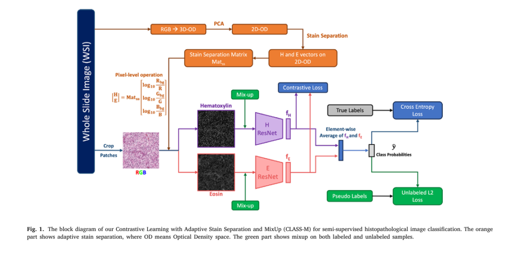
What Is CLASS-M? A New Era in Medical Image Analysis
Published in Medical Image Analysis, the paper titled “CLASS-M: Adaptive stain separation-based contrastive learning with pseudo-labeling for histopathological image classification” presents a novel approach to overcoming one of the biggest challenges in AI-driven pathology: the scarcity of labeled training data.
Traditional deep learning models require vast amounts of manually annotated images — a process that is time-consuming, expensive, and dependent on expert pathologists. CLASS-M solves this by leveraging semi-supervised learning, using a small set of labeled patches and a large pool of unlabeled whole slide images (WSIs) to train a highly accurate classifier.
CLASS-M stands for Contrastive Learning with Adaptive Stain Separation and MixUp, but it’s also a clever acronym for CLASSifying Medical images.
The model was tested on two ccRCC datasets:
- Utah ccRCC dataset: 49 WSIs with patch-level labels
- TCGA ccRCC dataset: 420 WSIs, with 150 labeled
Results showed CLASS-M achieved:
- 95.35% ± 0.46% test accuracy on the Utah dataset
- 92.13% ± 0.89% test accuracy on the TCGA dataset
These numbers surpass both supervised and self-supervised baselines — a true breakthrough in medical AI.
Why Patch-Level Classification Matters
Most AI models in histopathology use Multiple Instance Learning (MIL), which only requires slide-level labels (e.g., “cancer” or “normal”). While convenient, MIL has a critical limitation: it often focuses only on the most discriminative patches, leading to poor patch-level accuracy.
This is problematic when:
- Only a few cancerous regions exist in a large slide
- Local tumor grading is needed (e.g., low-risk vs. high-risk cancer)
- Necrotic or borderline regions must be identified
Patch-level classification, on the other hand, enables precise localization of cancerous tissue, helping pathologists:
- Reduce diagnostic time
- Improve consistency
- Catch early-stage cancers
CLASS-M delivers this precision — even with minimal labeled data.
How CLASS-M Works: 3 Key Innovations
1. Adaptive Stain Separation – Eliminating Color Variability
H&E-stained histopathological images vary widely due to differences in:
- Staining protocols
- Scanner types
- Laboratory conditions
To address this, CLASS-M uses adaptive stain separation based on the Macenko method (2009). Instead of using a fixed stain matrix, it computes a slide-specific stain matrix for each WSI, ensuring robustness across datasets.
🔍 Stain Separation Process:
- Convert RGB → Optical Density (OD) space:
where I0,C is the background intensity (e.g., 255), and IC is the pixel intensity.
- Apply PCA to find the 2D plane of H&E vectors.
- Estimate Hematoxylin (VH ) and Eosin (VE ) vectors.
- Reconstruct separated H and E images:
This process isolates nuclear (Hematoxylin) and cytoplasmic (Eosin) features — biologically meaningful channels for cancer detection.
2. Contrastive Learning on H & E Channels – Learning Shared Features
CLASS-M introduces a novel contrastive learning module that treats Hematoxylin and Eosin images as two independent views of the same tissue.
Using a Triplet Loss, the model pulls together features from the same patch while pushing apart features from different patches:
\[ L_{ct}(x_i) = \max\Big( \| f_H(x_i, H) – f_E(x_i, E) \|_2 – \| f_H(x_i, H) – f_E(x_k, E) \|_2 + m,\; 0 \Big) \]Where:
- fH,fE : ResNet encoders for H and E channels
- m : margin hyperparameter (optimized at 37)
- Positive pair: H and E from same patch
- Negative pair: H from one patch, E from another
This H/E contrastive learning forces the model to learn shared latent representations — improving generalization and robustness.
✅ Why not use RGB channels?
Ablation studies showed using Red/Green or Red/Blue as views performed 10–15% worse, proving that H and E are more independent and biologically relevant.
3. Pseudo-Labeling with MixUp – Boosting Performance on Small Datasets
To maximize the use of unlabeled data, CLASS-M uses pseudo-labeling and MixUp augmentation:
- Pseudo-labeling: Unlabeled patches are augmented K times, and their predictions are averaged and sharpened:
where T=0.5 controls label sharpness.
- MixUp: Labeled and pseudo-labeled samples are mixed:
This creates virtual training samples, improving regularization and performance — especially on rare classes like Necrosis.
💡 On the TCGA dataset, MixUp increased Necrosis accuracy from 60.47% to 86.65%.
Performance Comparison: CLASS-M vs. State-of-the-Art
| MODEL | UTAH CCRCC ACCURACY | TCGA CCRCC ACCURACY |
|---|---|---|
| ResNet (Supervised) | 88.85% | 72.11% |
| ViT (Supervised) | 84.69% | 73.50% |
| MoCo v3 (Self-Supervised) | 93.91% | 78.82% |
| SwAV (Self-Supervised) | 93.87% | 82.17% |
| FixMatch (Semi-Supervised) | 91.58% | 83.34% |
| MixMatch (Semi-Supervised) | 92.94% | 88.35% |
| CLASS (w/o MixUp) | 94.92% | 83.06% |
| CLASS-M (Ours) | 95.35% | 92.13% |
✅ CLASS-M outperforms all models on both datasets — a 3–10% improvement over existing methods.
Even compared to self-supervised models (which pre-train on unlabeled data), CLASS-M wins due to end-to-end semi-supervised training that jointly optimizes labeled and unlabeled data.
Ablation Studies: What Makes CLASS-M Work?
The authors conducted rigorous ablation studies to identify the contribution of each component:
| MODEL | UTAH ACCURACY | TCGA ACCURACY |
|---|---|---|
| CLASS-M (Full) | 95.35% | 92.13% |
| – Contrastive Loss | 90.92% | 89.70% |
| – RGB Augmentations | 94.41% | 91.21% |
| – Adaptive Stain Separation | 93.97% | 90.97% |
| – MixUp (CLASS) | 94.92% | 83.06% |
Key findings:
- Removing contrastive learning caused the biggest drop (~4–7%)
- Adaptive stain separation improved accuracy by 1–1.5%
- RGB augmentations before stain separation boosted performance
- MixUp added 9% gain on TCGA — critical for small-sample classes
Real-World Impact: Faster, More Accurate Cancer Diagnosis
CLASS-M isn’t just a lab experiment — it has real clinical value:
✅ Benefits:
- Reduces pathologist workload by highlighting suspicious regions
- Enables early detection of small cancer foci
- Works with minimal labeled data — ideal for rare cancers
- Generates prediction heatmaps for visual validation (see Appendix B)
❌ Limitations:
- Requires retraining for new tasks (less general than self-supervised models)
- Sensitive to staining artifacts and ink marks
- May misclassify ambiguous regions (e.g., inflammation vs. cancer)
Still, the 96.03% average pseudo-labeling accuracy (Appendix C) shows the model can reliably label unlabeled slides — reducing annotation burden.
Future Applications & Research Directions
CLASS-M’s framework is not limited to ccRCC. It can be applied to:
- Breast cancer (e.g., tumor grading in H&E slides)
- Prostate cancer (Gleason scoring)
- Immunohistochemistry (IHC) images
- Other stain types (e.g., PAS, Trichrome)
Future work could:
- Integrate noisy label handling for ambiguous regions
- Extend to 3D volumetric pathology
- Combine with explainable AI for clinical trust
- Deploy in real-time diagnostic pipelines
Call to Action: Join the AI Pathology Revolution
The CLASS-M model represents a paradigm shift in how we use AI in digital pathology. By combining adaptive stain separation, contrastive learning, and pseudo-labeling, it achieves unprecedented accuracy with minimal labeled data.
👉 Want to try CLASS-M yourself?
The code and annotations are publicly available on GitHub:
🔗 https://github.com/BzhangURU/Paper_CLASS-M
🧪 Researchers: Use the Utah ccRCC dataset (available via data transfer agreement) to benchmark your own models.
🏥 Hospitals: Explore integrating CLASS-M into your pathology workflow for faster, more accurate diagnoses.
🎓 Students: Study the ablation experiments and contrastive loss design — it’s a masterclass in medical AI engineering.
Conclusion: 1 Breakthrough, 1 Flaw, Infinite Potential
Breakthrough: CLASS-M sets a new benchmark in semi-supervised histopathological classification, proving that AI can achieve expert-level accuracy with minimal supervision.
Flaw: Current models still rely on patch-level annotations — a bottleneck that CLASS-M reduces but doesn’t eliminate.
Yet, the future is bright. With open-source code, strong performance, and biological interpretability, CLASS-M paves the way for AI-assisted pathology that is accurate, efficient, and scalable.
As kidney cancer affects 76,000+ people annually in the US, tools like CLASS-M could mean the difference between early detection and late-stage diagnosis.
The bottom line: CLASS-M isn’t just another AI model — it’s a life-saving innovation in the fight against cancer.
Here is a complete, self-contained Python script that implements the CLASS-M model using PyTorch.
# Full Python implementation of the CLASS-M model from the paper:
# "CLASS-M: Adaptive stain separation-based contrastive learning with
# pseudo-labeling for histopathological image classification"
#
# This script is self-contained and uses mock data for demonstration purposes.
#
# Dependencies:
# pip install torch torchvision scikit-learn numpy Pillow

import torch
import torch.nn as nn
import torch.optim as optim
import torchvision.models as models
import torchvision.transforms as T
from torch.utils.data import Dataset, DataLoader, Sampler
import numpy as np
from PIL import Image
from sklearn.decomposition import PCA
import torch.nn.functional as F
import random

# --- 1. Adaptive Stain Separation (Macenko et al., 2009) ---
# This section implements the unsupervised stain separation technique to
# get Hematoxylin (H) and Eosin (E) channels from an RGB image.

def rgb_to_od(im):
    """
    Converts an RGB image to Optical Density (OD) space.
    RGB -> OD = -log10(I / I_0)
    """
    im = im.astype(np.float64)
    # Set I_0 to 255, a common value for background intensity.
    I_0 = 255.0
    # Avoid division by zero or log of zero
    im[im == 0] = 1e-6
    return -1 * np.log10(im / I_0)

def get_stain_matrix(image, beta=0.15, alpha=1):
    """
    Calculates the stain matrix for an image based on the Macenko method.
    Args:
        image (np.array): An RGB image tile.
        beta (float): OD threshold for transparent pixels.
        alpha (int): Percentile for robust stain vector estimation.

    Returns:
        np.array: A 2x3 stain matrix for H and E.
    """
    # Convert from RGB to OD space
    od_image = rgb_to_od(image).reshape((-1, 3))

    # Filter out transparent pixels (clear background)
    od_filtered = od_image[np.all(od_image > beta, axis=1)]

    if od_filtered.shape[0] < 2:
        # Return a default matrix if not enough tissue is found
        # This is a common default for H&E
        return np.array([[0.5626, 0.7201, 0.4062],
                         [0.2159, 0.8012, 0.5581]])

    # Apply PCA to find the plane of the stains
    pca = PCA(n_components=2)
    principal_components = pca.fit_transform(od_filtered)

    # Project data onto the plane defined by the first two principal components
    # and find the angle of each point
    angles = np.arctan2(principal_components[:, 1], principal_components[:, 0])

    # Find the min and max angles
    min_angle = np.percentile(angles, alpha)
    max_angle = np.percentile(angles, 100 - alpha)

    # Convert angles back to vectors in the OD space
    vec1 = pca.components_.T @ np.array([np.cos(min_angle), np.sin(min_angle)])
    vec2 = pca.components_.T @ np.array([np.cos(max_angle), np.sin(max_angle)])

    # Order the vectors to ensure H is first, E is second
    if vec1[0] > vec2[0]:
        stain_vectors = np.array([vec1, vec2])
    else:
        stain_vectors = np.array([vec2, vec1])

    # Normalize vectors
    stain_vectors /= np.linalg.norm(stain_vectors, axis=1)[:, np.newaxis]

    return stain_vectors

# --- 2. Dataset and Dataloaders ---
# Custom Dataset to handle labeled and unlabeled data, and a balanced sampler.

class HistopathologyDataset(Dataset):
    def __init__(self, data, labels=None, transform=None, stain_matrix=None):
        """
        Args:
            data (list): List of image data (e.g., file paths or numpy arrays).
            labels (list, optional): List of labels. None for unlabeled data.
            transform (callable, optional): Optional transform to be applied on a sample.
            stain_matrix (np.array, optional): Pre-computed stain matrix.
        """
        self.data = data
        self.labels = labels
        self.is_labeled = labels is not None
        self.transform = transform
        self.stain_matrix = stain_matrix

    def __len__(self):
        return len(self.data)

    def __getitem__(self, idx):
        # In a real scenario, you would load an image from a path.
        # Here, we use the mock data directly.
        rgb_image = self.data[idx]

        # --- Stain Separation ---
        # If no global stain matrix is provided, compute it per image.
        # The paper suggests slide-level separation for consistency.
        if self.stain_matrix is None:
            current_stain_matrix = get_stain_matrix(np.array(rgb_image))
        else:
            current_stain_matrix = self.stain_matrix

        # Deconvolution
        od_image = rgb_to_od(np.array(rgb_image)).reshape((-1, 3))
        # Use pseudo-inverse for stability
        concentrations = np.linalg.pinv(current_stain_matrix.T) @ od_image.T

        # Separate H and E channels
        h_channel = concentrations[0, :].reshape(rgb_image.size[1], rgb_image.size[0])
        e_channel = concentrations[1, :].reshape(rgb_image.size[1], rgb_image.size[0])

        # Normalize for visualization and model input
        h_channel = (h_channel - h_channel.min()) / (h_channel.max() - h_channel.min() + 1e-6)
        e_channel = (e_channel - e_channel.min()) / (e_channel.max() - e_channel.min() + 1e-6)

        h_image = Image.fromarray((h_channel * 255).astype(np.uint8))
        e_image = Image.fromarray((e_channel * 255).astype(np.uint8))

        label = self.labels[idx] if self.is_labeled else -1

        if self.transform:
            rgb_image = self.transform['rgb'](rgb_image)
            h_image = self.transform['he'](h_image)
            e_image = self.transform['he'](e_image)

        return rgb_image, h_image, e_image, label

class BalancedSampler(Sampler):
    """
    Samples elements from a dataset with a balanced number of examples from each class.
    """
    def __init__(self, dataset):
        self.labels = np.array(dataset.labels)
        self.label_indices = {label: np.where(self.labels == label)[0]
                              for label in np.unique(self.labels)}
        self.num_samples = len(dataset)

    def __iter__(self):
        indices = []
        for _ in range(self.num_samples):
            label = random.choice(list(self.label_indices.keys()))
            idx = random.choice(self.label_indices[label])
            indices.append(idx)
        return iter(indices)

    def __len__(self):
        return self.num_samples

# --- 3. Model Architecture ---
# Dual ResNet18 encoders for H and E channels.

class CLASS_M_Model(nn.Module):
    def __init__(self, num_classes, pretrained=True):
        super(CLASS_M_Model, self).__init__()
        # --- H-channel Encoder ---
        self.h_encoder = models.resnet18(weights=models.ResNet18_Weights.IMAGENET1K_V1 if pretrained else None)
        # Adapt first layer for 1-channel (grayscale) input
        h_conv1_weight = self.h_encoder.conv1.weight.data.sum(dim=1, keepdim=True)
        self.h_encoder.conv1 = nn.Conv2d(1, 64, kernel_size=7, stride=2, padding=3, bias=False)
        self.h_encoder.conv1.weight.data = h_conv1_weight
        h_feature_dim = self.h_encoder.fc.in_features
        self.h_encoder.fc = nn.Identity() # Remove final layer

        # --- E-channel Encoder ---
        self.e_encoder = models.resnet18(weights=models.ResNet18_Weights.IMAGENET1K_V1 if pretrained else None)
        # Adapt first layer for 1-channel (grayscale) input
        e_conv1_weight = self.e_encoder.conv1.weight.data.sum(dim=1, keepdim=True)
        self.e_encoder.conv1 = nn.Conv2d(1, 64, kernel_size=7, stride=2, padding=3, bias=False)
        self.e_encoder.conv1.weight.data = e_conv1_weight
        e_feature_dim = self.e_encoder.fc.in_features
        self.e_encoder.fc = nn.Identity()

        # --- Classifier Head ---
        self.classifier = nn.Linear(h_feature_dim, num_classes)

    def forward(self, x_h, x_e):
        f_h = self.h_encoder(x_h)
        f_e = self.e_encoder(x_e)

        # Element-wise average of features as described in the paper
        f_avg = (f_h + f_e) / 2.0

        # Get class probabilities
        logits = self.classifier(f_avg)

        return logits, f_h, f_e

# --- 4. MixUp and Loss Functions ---

def sharpen(p, T):
    """Applies temperature sharpening to a probability distribution."""
    if p.dim() == 1:
        p = p.unsqueeze(0)
    pt = p**(1/T)
    return pt / pt.sum(dim=1, keepdim=True)

def mixup_data(x_h, x_e, y, alpha=1.0, device='cpu'):
    """Performs MixUp on a batch of data."""
    if alpha > 0:
        lam = np.random.beta(alpha, alpha)
    else:
        lam = 1

    batch_size = x_h.size()[0]
    index = torch.randperm(batch_size).to(device)

    lam = max(lam, 1 - lam) # As per paper's logic

    mixed_x_h = lam * x_h + (1 - lam) * x_h[index, :]
    mixed_x_e = lam * x_e + (1 - lam) * x_e[index, :]
    y_a, y_b = y, y[index]

    return mixed_x_h, mixed_x_e, y_a, y_b, lam

def triplet_loss(anchor, positive, negative, margin):
    """Calculates Triplet loss."""
    pos_dist = F.pairwise_distance(anchor, positive, p=2)
    neg_dist = F.pairwise_distance(anchor, negative, p=2)
    loss = torch.relu(pos_dist - neg_dist + margin)
    return loss.mean()

# --- 5. Main Training Loop ---
def train_model(config):
    device = torch.device("cuda" if torch.cuda.is_available() else "cpu")
    print(f"Using device: {device}")

    # --- Data Preparation ---
    # As per paper, augmentations are applied to RGB, H, and E images
    transformations = {
        'rgb': T.Compose([
            T.ColorJitter(brightness=0.4, contrast=0.4, saturation=0.4),
            T.ToTensor() # ToTensor is applied here to the original RGB
        ]),
        'he': T.Compose([
            T.RandomRotation(15),
            T.RandomHorizontalFlip(),
            T.RandomVerticalFlip(),
            # The paper crops to 256x256, we resize for simplicity
            T.Resize((224, 224)),
            T.ToTensor(),
            T.Normalize(mean=[0.5], std=[0.5]) # Normalize single channel images
        ])
    }

    # --- Mock Data Generation ---
    print("Generating mock data...")
    num_labeled = 128
    num_unlabeled = 512
    num_classes = 4 # e.g., Normal, Low Risk, High Risk, Necrosis

    # Labeled data
    labeled_images = [Image.fromarray(np.random.randint(0, 255, (256, 256, 3), dtype=np.uint8)) for _ in range(num_labeled)]
    labeled_labels = [random.randint(0, num_classes - 1) for _ in range(num_labeled)]

    # Unlabeled data
    unlabeled_images = [Image.fromarray(np.random.randint(0, 255, (256, 256, 3), dtype=np.uint8)) for _ in range(num_unlabeled)]

    # Create datasets
    labeled_dataset = HistopathologyDataset(labeled_images, labeled_labels, transform=transformations)
    unlabeled_dataset = HistopathologyDataset(unlabeled_images, labels=[0]*num_unlabeled, transform=transformations) # Dummy labels

    # Create dataloaders
    labeled_loader = DataLoader(labeled_dataset, batch_size=config['batch_size'] // 2, sampler=BalancedSampler(labeled_dataset))
    unlabeled_loader = DataLoader(unlabeled_dataset, batch_size=config['batch_size'] // 2, shuffle=True)

    # --- Model, Optimizer, and Loss ---
    model = CLASS_M_Model(num_classes=num_classes).to(device)
    optimizer = optim.Adam(model.parameters(), lr=config['learning_rate'])

    ce_loss_fn = nn.CrossEntropyLoss()
    l2_loss_fn = nn.MSELoss()

    print("Starting training...")
    for epoch in range(config['epochs']):
        model.train()

        # Use iterators to handle potentially different sized datasets
        labeled_iter = iter(labeled_loader)
        unlabeled_iter = iter(unlabeled_loader)

        total_loss = 0
        total_ce_loss = 0
        total_l2_loss = 0
        total_ct_loss = 0

        num_batches = min(len(labeled_loader), len(unlabeled_loader))

        for i in range(num_batches):
            try:
                # --- Get Data ---
                _, l_h, l_e, l_y = next(labeled_iter)
                _, u_h, u_e, _ = next(unlabeled_iter)

                l_h, l_e, l_y = l_h.to(device), l_e.to(device), l_y.to(device)
                u_h, u_e = u_h.to(device), u_e.to(device)

                # --- Pseudo-Labeling for Unlabeled Data ---
                with torch.no_grad():
                    # The paper uses K augmentations. For simplicity, we use one.
                    u_logits, _, _ = model(u_h, u_e)
                    u_probs = torch.softmax(u_logits, dim=1)
                    # Sharpen probabilities to create pseudo-labels
                    u_y_pseudo = sharpen(u_probs, T=config['sharpen_temp'])

                # --- Combine and MixUp ---
                all_h = torch.cat([l_h, u_h], dim=0)
                all_e = torch.cat([l_e, u_e], dim=0)
                all_y = torch.cat([F.one_hot(l_y, num_classes=num_classes).float(), u_y_pseudo], dim=0)

                mixed_h, mixed_e, y_a, y_b, lam = mixup_data(all_h, all_e, all_y, alpha=config['mixup_alpha'], device=device)

                # --- Forward Pass ---
                logits, f_h, f_e = model(mixed_h, mixed_e)

                # --- Loss Calculation ---
                # Split the mixed batch back into labeled and unlabeled portions
                labeled_batch_size = l_h.size(0)

                # Supervised Loss (Cross-Entropy)
                loss_ce = lam * ce_loss_fn(logits[:labeled_batch_size], y_a[:labeled_batch_size]) + \
                          (1 - lam) * ce_loss_fn(logits[:labeled_batch_size], y_b[:labeled_batch_size])

                # Unsupervised Loss (L2)
                pred_probs = torch.softmax(logits[labeled_batch_size:], dim=1)
                loss_l2 = lam * l2_loss_fn(pred_probs, y_a[labeled_batch_size:]) + \
                          (1 - lam) * l2_loss_fn(pred_probs, y_b[labeled_batch_size:])

                # Contrastive Loss (Triplet)
                # Create negative pairs by shuffling E-features
                shuffled_indices = torch.randperm(f_e.size(0)).to(device)
                f_e_negative = f_e[shuffled_indices]
                loss_ct = triplet_loss(f_h, f_e, f_e_negative, margin=config['contrastive_margin'])

                # --- Total Loss ---
                loss = loss_ce + config['lambda_u'] * loss_l2 + config['lambda_c'] * loss_ct

                # --- Backward Pass and Optimization ---
                optimizer.zero_grad()
                loss.backward()
                optimizer.step()

                total_loss += loss.item()
                total_ce_loss += loss_ce.item()
                total_l2_loss += loss_l2.item()
                total_ct_loss += loss_ct.item()

            except StopIteration:
                break

        avg_loss = total_loss / num_batches
        avg_ce = total_ce_loss / num_batches
        avg_l2 = total_l2_loss / num_batches
        avg_ct = total_ct_loss / num_batches

        print(f"Epoch [{epoch+1}/{config['epochs']}], Avg Loss: {avg_loss:.4f}, "
              f"CE Loss: {avg_ce:.4f}, L2 Loss: {avg_l2:.4f}, Contrastive Loss: {avg_ct:.4f}")

    print("Training finished.")


if __name__ == '__main__':
    # Hyperparameters from the paper and reasonable defaults
    config = {
        'epochs': 10,
        'batch_size': 32, # Paper uses 64
        'learning_rate': 1e-4,
        'sharpen_temp': 0.5,
        'mixup_alpha': 2.0,
        'lambda_u': 7.5, # Weight for unlabeled L2 loss
        'lambda_c': 0.1, # Weight for contrastive loss
        'contrastive_margin': 37.0
    }

    train_model(config)
Related posts, You May like to read
- 7 Shocking Truths About Knowledge Distillation: The Good, The Bad, and The Breakthrough (SAKD)
- 7 Revolutionary Breakthroughs in Medical Image Translation (And 1 Fatal Flaw That Could Derail Your AI Model)
- 7 Revolutionary Breakthroughs in Small Object Detection: The DAHI Framework
- 1 Revolutionary Breakthrough in AI Object Detection: GridCLIP vs. Two-Stage Models
Can you be more specific about the content of your article? After reading it, I still have some doubts. Hope you can help me. https://www.binance.com/sl/register?ref=GQ1JXNRE
I don’t think the title of your article matches the content lol. Just kidding, mainly because I had some doubts after reading the article. https://maribocares.org/2019/05/12/mental-health-cancer/