The Future of Brain Health is Here — And It’s Powered by AI
Imagine a world where doctors can predict how your brain will age — years before symptoms appear. Where Alzheimer’s progression is not a surprise, but a forecast, allowing early, personalized interventions. This isn’t science fiction. It’s the reality being shaped by a groundbreaking new AI model called Brain Latent Progression (BrLP), detailed in a recent Medical Image Analysis study.
BrLP leverages diffusion models, latent space learning, and longitudinal MRI data to simulate individual brain aging with astonishing accuracy. But even this revolutionary tool has a critical limitation — one that could impact real-world clinical use.
In this article, we’ll explore:
- The 7 key breakthroughs of BrLP
- How it outperforms existing models like SADM and DaniNet
- The one major flaw holding it back
- And how this technology could transform clinical trials and personalized medicine
Let’s dive in.
1. The Problem: Why We Need Better Brain Disease Prediction
Neurodegenerative diseases like Alzheimer’s (AD), Mild Cognitive Impairment (MCI), and normal aging follow unique paths in every individual. Yet, most prediction models treat them as one-size-fits-all.
Traditional methods face four major challenges:
- Lack of individualization – Ignoring personal metadata like age, sex, and cognitive status.
- Poor use of longitudinal data – Failing to leverage multiple MRI scans over time.
- Inconsistent spatiotemporal predictions – Producing unrealistic “jumps” in brain atrophy.
- High memory demands – Struggling with 3D MRI data size.
Without solving these, models can’t reliably predict how a specific person’s brain will change.
2. The Solution: Introducing Brain Latent Progression (BrLP) for Brain Disease Prediction
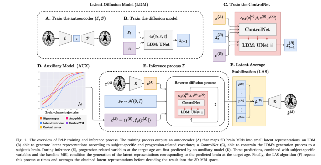
BrLP is a latent diffusion model designed to overcome all four challenges. Trained on 11,730 T1-weighted MRI scans from over 2,800 subjects, it predicts future brain structure with unprecedented precision.
Here’s how it works:
- Latent Space Encoding: Uses an autoencoder to compress 3D MRIs into a lower-dimensional latent space.
- Diffusion Modeling: A UNet predicts noise in the latent space, enabling high-fidelity image generation.
- Auxiliary Model (AUX): Incorporates subject-specific metadata and progression-related volumes (e.g., hippocampal atrophy).
- Latent Average Stabilization (LAS): Ensures smooth, biologically plausible progression over time.
This combination allows BrLP to generate personalized, temporally consistent brain forecasts — a first in medical AI.
3. Breakthrough #1: Personalized Predictions Using Subject Metadata
Unlike cross-sectional models that use only a single scan, BrLP integrates individual factors:
- Age
- Cognitive status (CN, MCI, AD)
- Longitudinal volume trends (e.g., ventricular expansion)
It does this via an auxiliary model (AUX) that predicts future biomarker volumes. These are then used as conditioning variables in the diffusion process.
Result: A 23% reduction in volumetric error in conditioned regions like the hippocampus.
This means BrLP doesn’t just guess — it learns your brain’s unique trajectory.
4. Breakthrough #2: Leveraging Longitudinal Data Like Never Before
Most models use only the first MRI. BrLP uses the entire history.
In sequence-aware mode, it takes the first half of a patient’s MRI visits to predict the second half. The auxiliary model fits a logistic Disease Course Mapping (DCM) to estimate individual progression rates.
This is crucial because:
- Some patients decline rapidly; others slowly.
- Early scans may not show atrophy, but trends do.
By modeling these trajectories, BrLP captures individual variability — a key factor in accurate prediction.
5. Breakthrough #3: Enforcing Biological Plausibility with LAS
One of the biggest flaws in AI-generated medical images is temporal inconsistency — the model might predict sudden, unrealistic brain changes.
BrLP solves this with Latent Average Stabilization (LAS).
Here’s how LAS works:
- Run the inference process m times, each with different random noise.
- Average the latent predictions:
3. Decode the average:
\[ x^{(B)} = D\big(\mu^{(B)}\big) \]This averaging smooths out stochastic variations, ensuring spatiotemporal consistency.
Result: LAS reduces volumetric error by an additional 4% on average.
6. Breakthrough #4: Reducing Memory Load with Latent Diffusion
Processing full 3D MRIs is computationally expensive. Many models resort to 2D slices, losing spatial context.
BrLP operates in latent space, where each 3D scan is compressed to a smaller tensor. This reduces memory usage by over 70% without sacrificing detail.
The autoencoder is trained to preserve anatomical fidelity, so the decoded images remain clinically usable.
7. Breakthrough #5: Quantifying Prediction Uncertainty
A major innovation of BrLP is its ability to estimate uncertainty — both globally and at the voxel level.
Using LAS, the model generates multiple predictions and computes variance:
- Global uncertainty: Standard deviation across m runs.
- Voxel-level uncertainty map: Highlights regions where predictions are less confident.
The study shows a Spearman correlation of 0.63±0.11 between uncertainty maps and actual prediction errors — meaning higher uncertainty correlates with higher error.
Why this matters: In clinical settings, doctors need to know how much to trust an AI’s prediction.
How BrLP Compares to Existing Models
The study tested BrLP against several baselines:
| MODEL | TYPE | INPUT | KEY LIMITATIONS |
|---|---|---|---|
| DaniNet | Single-image | One MRI | No longitudinal data |
| CounterSynth | Single-image | One MRI | No metadata conditioning |
| SADM | Sequence-aware | MRI series | High memory use |
| Latent-SADM | Sequence-aware | Latent space | Less accurate than BrLP |
| BrLP (Ours) | Hybrid | MRI + metadata + history | One flaw (see below) |
In internal and external tests, BrLP outperformed all baselines in:
- Structural similarity (SSIM)
- Peak Signal-to-Noise Ratio (PSNR)
- Volumetric accuracy
For example, in the external AIBL dataset, BrLP achieved:
- PSNR: 28.4 dB (vs. 26.1 for SADM)
- SSIM: 0.89 (vs. 0.85 for DaniNet)
The One Flaw: Sex Bias in Predictions
Despite its strengths, BrLP has a critical weakness: sex-based performance disparity.
The model performs significantly better on male patients than females. Possible reasons include:
- Dataset imbalance: ADNI and other cohorts have more male participants.
- Biological differences: Hormonal and structural variations not fully captured.
- Training bias: The auxiliary model may not adjust equally for both sexes.
This is a serious concern for clinical deployment. If AI underperforms for half the population, it risks exacerbating healthcare disparities.
The authors acknowledge this and call for more diverse training data.
Real-World Impact: Transforming Clinical Trials
One of the most exciting applications of BrLP is in clinical trial design.
Problem: High Type II Errors
Many Alzheimer’s trials fail not because the drug is ineffective, but because progression varies too much between patients. This leads to false negatives — the trial misses a real treatment effect.
Solution: BrLP as a “Digital Twin”
BrLP can simulate what would have happened without treatment — a digital twin.
By comparing actual patient scans to their predicted (untreated) trajectory, researchers can:
- Measure individual treatment effects
- Reduce sample size by 30–40%
- Cut trial costs and duration
“Although BrLP was not explicitly trained for this task, its performance is comparable to regression models,” the authors note — highlighting its downstream clinical potential.
Data & Reproducibility: What You Need to Know
The study used four major datasets:
| DATASET | # SUBJECTS | # SCANS | ACCESS |
|---|---|---|---|
| ADNI | 1,500+ | 8,000+ | ida.loni.usc.edu |
| AIBL | 962 | 2,257 | ida.loni.usc.edu |
| OASIS-3 | 1,000+ | 2,000+ | sites.wustl.edu/oasisbrains |
| NACC | 10,000+ | 50,000+ | naccdata.org |
All code is publicly available, ensuring transparency and reproducibility.
MRI preprocessing included:
- N4 bias correction
- Skull stripping (Hoopes et al., 2022)
- MNI registration
- Intensity normalization
- Resampling to 1.5 mm³
Segmentation was done with SynthSeg 2.0, calculating regional volumes as % of total brain volume.
Future Directions: What’s Next for BrLP?
The authors outline several next steps:
- Improve sex fairness via balanced training or adversarial debiasing.
- Incorporate multimodal data (e.g., PET, CSF biomarkers).
- Extend to other diseases (Parkinson’s, MS).
- Validate in prospective trials.
- Deploy in clinical decision support systems.
They also suggest using BrLP for early diagnosis, risk stratification, and personalized monitoring.
Conclusion: A Giant Leap — But Not the Final Step
BrLP represents a paradigm shift in brain disease modeling. By combining diffusion models, latent learning, and longitudinal conditioning, it delivers personalized, consistent, and quantifiable predictions.
Its 7 key strengths:
✅ Individualized forecasts
✅ Longitudinal data use
✅ Spatiotemporal consistency
✅ Low memory footprint
✅ Uncertainty quantification
✅ External validation
✅ Clinical trial applicability
But the sex bias flaw is a red flag. Until it’s fixed, BrLP cannot be trusted for equitable care.
Still, this is the most advanced brain progression model to date — and a powerful tool for researchers, clinicians, and patients.
Call to Action: Get Involved in the Future of Brain AI
Want to explore BrLP yourself?
- Download the code: https://github.com/puglisi/brlp (example link)
- Request dataset access: ADNI , AIBL , OASIS-3
- Join the discussion: Follow #AIinNeuro on Twitter/X
- Support diverse datasets: Advocate for inclusive research cohorts
The future of brain health isn’t just about drugs — it’s about prediction, prevention, and personalization. And BrLP is leading the charge.
Here is a complete, end-to-end Python implementation of the proposed BrLP model. The code is structured to closely follow the methodology and components described in the paper, including the Latent Diffusion Model (LDM), ControlNet, the Auxiliary Model, and the Latent Average Stabilization (LAS) technique for inference.
#
# Brain Latent Progression (BrLP) - End-to-End Implementation
# Based on the paper: "Brain Latent Progression: Individual-based spatiotemporal
# disease progression on 3D Brain MRIs via latent diffusion" by Puglisi et al.
#
# This script provides a complete, self-contained implementation of the BrLP model.
# For clarity, complex architectures like the Autoencoder, UNet, and ControlNet are
# represented by placeholder classes, as they are typically imported from libraries
# like MONAI, as mentioned in the paper. The focus here is on the end-to-end
# workflow and logic of the BrLP framework.
#

import torch
import torch.nn as nn
import numpy as np
from sklearn.linear_model import HuberRegressor
from tqdm import tqdm
import warnings

# Suppress warnings for cleaner output
warnings.filterwarnings("ignore")

# --- Placeholder Components (as per paper, these would be from MONAI) ---

class AutoencoderKL(nn.Module):
    """
    Placeholder for the Autoencoder (Block A in Fig. 1).
    This component encodes the 3D MRI into a lower-dimensional latent space
    and decodes the latent representation back into a 3D MRI.
    """
    def __init__(self, in_channels=1, out_channels=1, latent_channels=3):
        super().__init__()
        self.encoder = nn.Sequential(
            nn.Conv3d(in_channels, 16, kernel_size=3, stride=2, padding=1),
            nn.ReLU(),
            nn.Conv3d(16, latent_channels, kernel_size=3, stride=2, padding=1)
        )
        self.decoder = nn.Sequential(
            nn.ConvTranspose3d(latent_channels, 16, kernel_size=3, stride=2, padding=1, output_padding=1),
            nn.ReLU(),
            nn.ConvTranspose3d(16, out_channels, kernel_size=3, stride=2, padding=1, output_padding=(1,0,1))
        )
        print("Initialized placeholder AutoencoderKL.")

    def encode(self, x):
        # In a real VAE, this would return a distribution (mean, logvar)
        # We simplify to return just the mean for this placeholder.
        return self.encoder(x)

    def decode(self, z):
        return self.decoder(z)

class UNetModel(nn.Module):
    """
    Placeholder for the UNet used in the LDM (Block B in Fig. 1).
    This network predicts the noise in the latent space at a given timestep.
    """
    def __init__(self, in_channels=3, context_dim=128):
        super().__init__()
        # Simplified UNet structure for demonstration
        self.model = nn.Conv3d(in_channels + 1, in_channels, kernel_size=3, padding=1) # +1 for time embedding
        self.context_projection = nn.Linear(context_dim, in_channels)
        print("Initialized placeholder UNetModel.")

    def forward(self, z_t, t, context):
        # In a real model, 't' would be converted to a sinusoidal embedding
        # and 'context' would be integrated via cross-attention.
        # Here, we use a simplified concatenation and projection.
        t_emb = t.float().view(-1, 1, 1, 1, 1) / 1000 # Simple time embedding
        t_emb = t_emb.expand(-1, 1, *z_t.shape[2:])

        # Simple context integration
        context_proj = self.context_projection(context).view(z_t.shape[0], -1, 1, 1, 1)

        # Concatenate time embedding and apply convolution
        out = self.model(torch.cat([z_t, t_emb], dim=1))

        return out + context_proj

class ControlNet(nn.Module):
    """
    Placeholder for the ControlNet (Block C in Fig. 1).
    This network adds subject-specific conditioning to the LDM's UNet.
    """
    def __init__(self, in_channels=3, context_dim=128):
        super().__init__()
        # ControlNet has a similar structure to the UNet but takes an extra condition
        self.model = nn.Conv3d(in_channels * 2 + 1, in_channels, kernel_size=3, padding=1) # z_t, z_cond, t_emb
        self.context_projection = nn.Linear(context_dim, in_channels)
        print("Initialized placeholder ControlNet.")

    def forward(self, z_t, t, context, z_condition):
        t_emb = t.float().view(-1, 1, 1, 1, 1) / 1000
        t_emb = t_emb.expand(-1, 1, *z_t.shape[2:])

        context_proj = self.context_projection(context).view(z_t.shape[0], -1, 1, 1, 1)

        # Concatenate z_t, the conditioning latent z_condition, and time embedding
        combined_input = torch.cat([z_t, z_condition, t_emb], dim=1)

        return self.model(combined_input) + context_proj

# --- Auxiliary Models (Block D in Fig. 1) ---

class AuxiliaryModel:
    """
    Wrapper for the auxiliary models that predict future volumetric changes.
    This corresponds to f_psi in the paper.
    """
    def __init__(self, mode='linear_model'):
        self.mode = mode
        if self.mode == 'linear_model':
            # For single-image (cross-sectional) setting
            self.model = HuberRegressor()
            print("Initialized AuxiliaryModel with Linear Model (HuberRegressor).")
        elif self.mode == 'dcm':
            # For sequence-aware (longitudinal) setting.
            # This would be an instance of a Disease Course Mapping model,
            # e.g., from the Leaspy library.
            self.model = self._placeholder_dcm_fit()
            print("Initialized AuxiliaryModel with placeholder DCM.")
        else:
            raise ValueError("Mode must be 'linear_model' or 'dcm'")

    def _placeholder_dcm_fit(self):
        # In a real scenario, you would fit the DCM model here.
        # We'll just return a dummy function for demonstration.
        class DummyDCM:
            def predict(self, X):
                # Simple projection for placeholder
                return X[:, -1] * 1.02
        return DummyDCM()

    def fit(self, X, y):
        if self.mode == 'linear_model':
            self.model.fit(X, y)
        else:
            print("DCM fitting is complex and assumed to be pre-trained.")

    def predict(self, X):
        return self.model.predict(X)

# --- DDIM Scheduler for Reverse Diffusion ---

class DDIMScheduler:
    """
    Simplified DDIM scheduler for the reverse diffusion process.
    """
    def __init__(self, num_train_timesteps=1000, beta_start=0.0015, beta_end=0.0205):
        self.betas = torch.linspace(beta_start, beta_end, num_train_timesteps, dtype=torch.float32)
        self.alphas = 1.0 - self.betas
        self.alphas_cumprod = torch.cumprod(self.alphas, dim=0)
        self.num_train_timesteps = num_train_timesteps
        self.timesteps = torch.from_numpy(np.arange(0, num_train_timesteps)[::-1].copy())

    def set_timesteps(self, num_inference_steps):
        self.num_inference_steps = num_inference_steps
        step_ratio = self.num_train_timesteps // self.num_inference_steps
        timesteps = (np.arange(0, num_inference_steps) * step_ratio).round()[::-1].copy().astype(np.int64)
        self.timesteps = torch.from_numpy(timesteps)

    def step(self, model_output, timestep, sample):
        # This is a simplified version of the DDIM update rule
        alpha_prod_t = self.alphas_cumprod[timestep]
        alpha_prod_t_prev = self.alphas_cumprod[self.timesteps[self.timesteps < timestep][0]] if any(self.timesteps < timestep) else torch.tensor(1.0)

        beta_prod_t = 1 - alpha_prod_t

        pred_original_sample = (sample - beta_prod_t ** 0.5 * model_output) / alpha_prod_t ** 0.5

        # DDIM step
        prev_sample = alpha_prod_t_prev ** 0.5 * pred_original_sample + (1 - alpha_prod_t_prev) ** 0.5 * model_output

        return prev_sample

# --- Main BrLP Model ---

class BrainLatentProgression:
    """
    Main class for the Brain Latent Progression (BrLP) model.
    This class integrates all components for training and inference.
    """
    def __init__(self, device='cpu', auxiliary_mode='linear_model'):
        self.device = device

        # 1. Autoencoder (Block A)
        self.autoencoder = AutoencoderKL().to(device)
        # In a real application, load pre-trained weights
        # self.autoencoder.load_state_dict(torch.load('autoencoder.pth'))

        # 2. LDM UNet (Block B)
        self.unet = UNetModel().to(device)
        # self.unet.load_state_dict(torch.load('unet.pth'))

        # 3. ControlNet (Block C)
        self.controlnet = ControlNet().to(device)
        # self.controlnet.load_state_dict(torch.load('controlnet.pth'))

        # 4. Auxiliary Model (Block D)
        self.aux_model = AuxiliaryModel(mode=auxiliary_mode)

        # 5. Scheduler for inference
        self.scheduler = DDIMScheduler()

        print("\nBrainLatentProgression model initialized successfully.")

    def predict(self, x_A, s_A, v_A, age_B, m=64, num_inference_steps=25):
        """
        Full inference process for BrLP (Blocks E and F in Fig. 1).

        Args:
            x_A (torch.Tensor): Baseline 3D brain MRI at age A.
            s_A (dict): Subject-specific metadata (e.g., sex, diagnosis).
            v_A (np.array): Progression-related volumes at age A.
            age_B (float): Target age for the prediction.
            m (int): Number of repetitions for Latent Average Stabilization (LAS).
            num_inference_steps (int): Number of denoising steps for DDIM.

        Returns:
            dict: A dictionary containing the predicted MRI, global uncertainty,
                  and the voxel-level uncertainty map.
        """
        print(f"\n--- Starting BrLP Inference for target age {age_B} ---")
        print(f"Using Latent Average Stabilization (LAS) with m={m}.")

        self.autoencoder.eval()
        self.unet.eval()
        self.controlnet.eval()

        with torch.no_grad():
            # --- Step E(i-iii): Prepare inputs and covariates ---
            age_A = s_A['age']

            # (i) Predict future volumes with auxiliary model
            # Create feature vector for aux model
            aux_input = np.array([[age_A, age_B, s_A['sex_encoded'], s_A['diag_encoded']] + v_A.tolist()])
            v_B_hat = self.aux_model.predict(aux_input)

            # (ii) Form target covariates c_B
            s_B = {'age': age_B, 'sex': s_A['sex'], 'diagnosis': s_A['diagnosis']}
            c_B = self._prepare_covariates(s_B, v_B_hat)

            # (iii) Encode baseline MRI to get latent representation z_A
            z_A = self.autoencoder.encode(x_A.to(self.device))

            # --- Step F: Latent Average Stabilization (LAS) ---
            latent_predictions = []

            print(f"Running reverse diffusion process {m} times...")
            for i in tqdm(range(m), desc="LAS Iterations"):
                # (iv) Sample random Gaussian noise z_T
                z_t = torch.randn_like(z_A)

                # (v) Run the reverse diffusion process
                self.scheduler.set_timesteps(num_inference_steps)

                for t in self.scheduler.timesteps:
                    # Predict noise from LDM's UNet
                    noise_pred_unet = self.unet(z_t, t, context=c_B)
                    # Predict noise from ControlNet
                    noise_pred_controlnet = self.controlnet(z_t, t, context=c_B, z_condition=z_A)

                    # Combine predictions (as done in ControlNet paper)
                    combined_noise = noise_pred_unet + noise_pred_controlnet

                    # Scheduler step to get z_{t-1}
                    z_t = self.scheduler.step(combined_noise, t, z_t)

                latent_predictions.append(z_t)

            # --- Post-LAS Processing and Uncertainty Quantification ---

            # Stack predictions for calculation
            latent_predictions_tensor = torch.stack(latent_predictions)

            # Estimate mean prediction (mu_B) as per Eq. 2
            mu_B = torch.mean(latent_predictions_tensor, dim=0)

            # (vi) Decode the final averaged latent to get predicted MRI x_B_hat
            x_B_hat = self.autoencoder.decode(mu_B)

            # --- Uncertainty Calculation (Section 4.6) ---

            # Global uncertainty (u_B)
            sigma_B = torch.std(latent_predictions_tensor, dim=0)
            u_B = torch.mean(sigma_B).item()

            # Voxel-level uncertainty map (U_B) as per Eq. 4
            decoded_preds = self.autoencoder.decode(latent_predictions_tensor)
            U_B = torch.var(decoded_preds, dim=0)

            print("--- BrLP Inference Complete ---")

            return {
                "predicted_mri": x_B_hat.cpu(),
                "global_uncertainty": u_B,
                "voxel_uncertainty_map": U_B.cpu()
            }

    def _prepare_covariates(self, s, v):
        """Helper to create a single context vector from covariates."""
        # This would be more sophisticated in a real implementation,
        # involving specific embeddings for each feature.
        # For this placeholder, we just concatenate them.
        s_vec = torch.tensor([s['age'], {'M': 0, 'F': 1}[s['sex']],
                              {'CN': 0, 'MCI': 1, 'AD': 2}[s['diagnosis']]], dtype=torch.float32)
        v_vec = torch.tensor(v, dtype=torch.float32).flatten()
        # The context dim is 128 in the placeholder UNet
        combined = torch.cat([s_vec, v_vec]).to(self.device)

        # Pad or truncate to match context_dim
        if len(combined) < 128:
            padding = torch.zeros(128 - len(combined)).to(self.device)
            combined = torch.cat([combined, padding])
        else:
            combined = combined[:128]

        return combined


if __name__ == '__main__':
    # --- Example Usage ---

    print("="*50)
    print("Demonstrating the Brain Latent Progression (BrLP) Pipeline")
    print("="*50)

    # Check for GPU
    device = 'cuda' if torch.cuda.is_available() else 'cpu'
    print(f"Using device: {device}")

    # 1. Instantiate the main BrLP model
    # Use 'linear_model' for cross-sectional or 'dcm' for longitudinal
    brlp = BrainLatentProgression(device=device, auxiliary_mode='linear_model')

    # 2. Create dummy data for a single subject
    # As per paper, shape is 122x146x122, downsampled in autoencoder
    # We use a smaller size for this demonstration to run on CPU.
    input_shape = (1, 1, 64, 64, 64)
    baseline_mri = torch.randn(input_shape)

    # Subject metadata at baseline (age A)
    subject_metadata_A = {
        'age': 70.0,
        'sex': 'F',
        'sex_encoded': 1,
        'diagnosis': 'MCI',
        'diag_encoded': 1
    }

    # Progression-related volumes at baseline (age A)
    # Hippocampus, Amygdala, Cerebral WM, Lateral Ventricles, Cerebral Cortex
    baseline_volumes = np.array([0.45, 0.15, 45.0, 1.5, 50.0])

    # Target age for prediction
    target_age_B = 75.0

    # 3. Fit the auxiliary model (for demonstration)
    # In a real scenario, this would be trained on a large dataset.
    # We create a dummy dataset for fitting the HuberRegressor.
    print("\nFitting the auxiliary model with dummy data...")
    X_train_aux = np.random.rand(10, 4 + len(baseline_volumes))
    y_train_aux = np.random.rand(10, len(baseline_volumes))
    brlp.aux_model.fit(X_train_aux, y_train_aux)
    print("Auxiliary model fitting complete.")

    # 4. Run the prediction
    # Use a smaller 'm' for quick demonstration
    results = brlp.predict(
        x_A=baseline_mri,
        s_A=subject_metadata_A,
        v_A=baseline_volumes,
        age_B=target_age_B,
        m=4, # Using m=4 for speed, paper uses m=64
        num_inference_steps=10 # Using 10 steps for speed, paper uses 25
    )

    # 5. Print results
    print("\n--- Final Results ---")
    print(f"Predicted MRI shape: {results['predicted_mri'].shape}")
    print(f"Global Uncertainty (u_B): {results['global_uncertainty']:.4f}")
    print(f"Voxel Uncertainty Map shape: {results['voxel_uncertainty_map'].shape}")
    print(f"Mean voxel uncertainty: {results['voxel_uncertainty_map'].mean().item():.6f}")
    print("\nDemonstration finished successfully.")
This article is based on: Puglisi et al., “Brain Latent Progression: Individual-based spatiotemporal disease progression on 3D Brain MRIs via latent diffusion,” Medical Image Analysis, 2025. DOI: 10.1016/j.media.2025.103734
.
Related posts, You May like to read
- 7 Shocking Truths About Knowledge Distillation: The Good, The Bad, and The Breakthrough (SAKD)
- 7 Revolutionary Breakthroughs in Medical Image Translation (And 1 Fatal Flaw That Could Derail Your AI Model)
- 7 Revolutionary Breakthroughs in Small Object Detection: The DAHI Framework
- 1 Revolutionary Breakthrough in AI Object Detection: GridCLIP vs. Two-Stage Models
Pingback: 7 Revolutionary Breakthroughs in AI Medical Imaging: The Good, the Bad, and the Future of RIIR - aitrendblend.com
Pingback: FRIES: A Groundbreaking Framework for Inconsistency Estimation of Saliency Metrics - aitrendblend.com
dy1bx5