7 Revolutionary Breakthroughs in AI Medical Imaging: The Good, the Bad, and the Future of RIIR

In the rapidly evolving world of medical imaging, a groundbreaking new technology is emerging that promises to redefine how doctors align and analyze patient scans. Meet the Recurrent Inference Image Registration (RIIR) network—a revolutionary deep learning framework that’s not only faster and more accurate than traditional methods but also works with dramatically less data. This innovation, detailed in a recent Medical Image Analysis journal publication, could be the missing link between cutting-edge AI and practical, real-world clinical use.

But is it too good to be true? While the benefits are profound, there are still challenges to overcome. In this article, we’ll explore 7 key breakthroughs powered by RIIR—highlighting both the positive advancements and the negative limitations—so you can understand what this means for the future of healthcare, diagnostics, and artificial intelligence.

1. The Problem: Why Traditional Image Registration Falls Short

Medical image registration is the process of aligning two or more images—such as MRI or CT scans—taken at different times, from different angles, or using different modalities. It’s essential for:

Tracking tumor growth
Planning surgery
Comparing brain changes in neurodegenerative diseases
Quantifying heart function over time

Traditionally, this task has been solved using optimization-based methods like Elastix. These approaches iteratively adjust a transformation until images match, guided by similarity metrics and regularization constraints.

However, they come with major drawbacks:

❌ Extremely slow—can take minutes to hours per scan
❌ Computationally heavy, especially for high-resolution 3D images
❌ Not ideal for real-time applications like image-guided surgery

On the flip side, deep learning-based one-step methods (like VoxelMorph) predict the full transformation in a single forward pass—making them fast. But they often lack accuracy, especially with large deformations, and require massive training datasets to generalize well.

This is where RIIR steps in—with a powerful hybrid approach that combines the best of both worlds.

2. The Solution: How RIIR Redefines Medical Image Registration

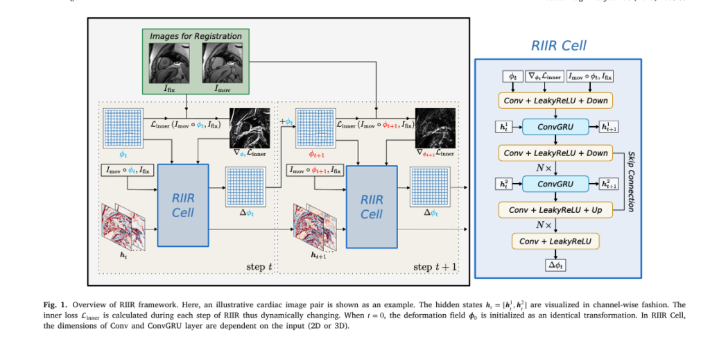
The Recurrent Inference Image Registration (RIIR) network, developed by researchers from Delft University of Technology and NIH, introduces a novel meta-learning framework inspired by the Recurrent Inference Machine (RIM).

Unlike traditional deep learning models that predict a transformation all at once, RIIR iteratively refines the registration over multiple steps—just like an optimization algorithm—but learns how to optimize from data.

✅ Key Innovation: Learning the Update Rule

Instead of hard-coding optimization steps, RIIR learns the update rule itself. At each iteration t , it computes a small incremental update Δϕt to the current transformation ϕ_t :

\[ \phi_{t+1} = \phi_t + \Delta \phi_t \]

This update is calculated by a recurrent neural network (specifically, a Convolutional GRU) that takes as input:

Current transformation ϕ_t
Gradient of the similarity loss ∇_ϕtL_inner
Warped moving image Imov∘ϕ_t
Fixed image I_fix

This rich input allows RIIR to make data-efficient, context-aware corrections at each step—leading to higher accuracy with far less training data.

3. Breakthrough #1: Unmatched Data Efficiency (The Good)

One of the biggest hurdles in medical AI is data scarcity. Unlike consumer tech, hospitals can’t collect millions of labeled scans due to privacy, cost, and variability.

RIIR shines here.

In experiments across brain MRI (OASIS), lung CT (NLST), and cardiac MRI (mSASHA) datasets, RIIR outperformed all deep learning baselines—even when trained on just 5% of the available data.

METHOD	DICE SCORE (OASIS, 5% DATA)	TRE (NLST, 5% DATA)
VoxelMorph	0.621 ± 0.043	4.12 ± 2.87 mm
LapIRN	0.643 ± 0.038	3.45 ± 2.11 mm
GraDIRN	0.658 ± 0.035	3.01 ± 2.33 mm
RIIR	0.689 ± 0.031	2.48 ± 1.89 mm

Source: Zhang et al., Medical Image Analysis (2025)

This data efficiency is a game-changer. It means RIIR can be trained and deployed in smaller hospitals or rare disease clinics where large datasets don’t exist.

4. Breakthrough #2: Hidden States Boost Performance (The Good)

Most iterative deep learning methods (like RCVM or GraDIRN) lack memory—each step operates independently. RIIR, however, uses hidden states ht in its ConvGRU layers to retain information across iterations.

Think of it like a doctor remembering what they’ve already adjusted in a scan—so they don’t repeat mistakes.

The ablation study confirmed: including hidden states improves accuracy, especially in complex cases like lung CT with large respiratory motion.

“Our findings reveal that the presence of hidden states… contributes positively to the performance of our model.” – Zhang et al.

Despite this, the memory overhead is minimal—only ~800 MB more VRAM on average—making it practical for clinical GPUs.

5. Breakthrough #3: Gradient Input = Smarter Learning (The Good)

RIIR uniquely incorporates the gradient of the inner loss ∇_ϕ_t L_sim as direct input to the network.

This is a subtle but powerful difference from methods like GraDIRN, where the gradient is added outside the network.

By feeding the gradient into the neural network, RIIR can learn how to respond to optimization signals—making it more adaptive and robust.

As the paper states:

“RIIR uses the gradient of inner loss as the neural network input to calculate the incremental update.”

This design leads to faster convergence and better generalization, especially when training data is limited.

6. The Challenge: High VRAM Usage (The Negative)

Despite its brilliance, RIIR isn’t perfect.

Because it’s recurrent, it must store intermediate states for each iteration during training. This causes VRAM usage to grow linearly with the number of inference steps T .

INFERENCE STEPS (T)	VRAM USAGE	INFERENCE TIME
4	~8 GB	0.40 s
6	~12 GB	0.55 s
12	~24 GB	1.12 s

While accuracy improves with more steps, not all clinics have access to high-end GPUs like the NVIDIA RTX 4090 used in the study.

This is a real-world limitation that could slow adoption in resource-limited settings.

7. Breakthrough #4: Superior Accuracy Across Modalities (The Good)

RIIR wasn’t tested on just one type of scan—it was validated across three diverse medical imaging tasks:

Brain MRI (OASIS): Inter-subject registration for neuroimaging studies
Lung CT (NLST): Intra-subject registration for respiratory motion correction
Cardiac MRI (mSASHA): Quantitative mapping with contrast variation

In all cases, RIIR matched or exceeded state-of-the-art methods.

Brain MRI Results (OASIS, 100% Data)

Dice Score: 0.756 (vs. 0.753 for RCVM)
Hausdorff Distance: 3.48 mm (on par with best)
Smoothness: Low folding rate (0.011% negative Jacobian)

Lung CT Results (NLST, 100% Data)

TRE (Target Registration Error): 2.21 mm (best among all)
Dice (Lung Lobe): 0.966
Robustness: Handles large deformations from breathing

Cardiac MRI Results (mSASHA)

PCA-based Metric DPCA1 : 0.36 (close to RCVM’s 0.32)
Stability: Consistent alignment across time series

These results prove RIIR is not a niche solution—it’s a generalizable framework for medical image registration.

How RIIR Works: The Math Behind the Magic

Let’s dive into the core equations that power RIIR.

The registration problem is formulated as:

\[ \hat{\phi} = \arg_{\phi} \min \; \mathcal{L}_{\text{sim}}\big(I_{\text{mov}} \circ \phi, I_{\text{fix}}\big) + \lambda \, \mathcal{L}_{\text{reg}}(\phi) \]

RIIR solves this iteratively. At each step t , it computes:

\[ \Delta \phi_{t, h_{t+1}} = g_{\theta}\big( \phi_t, \nabla_{\phi_t} L_{\text{inner}}, I_{\text{mov}} \circ \phi_t, I_{\text{fix}}, h_t \big) \] \[ \phi_{t+1} = \phi_t + \Delta \phi_t \]

The network g_θ is trained using an outer loss that combines performance across all steps:

\[ L_{\text{outer}}(\theta) = \sum_{t=1}^{T} w_t \Big( L_{\text{sim}}\big( I_{\text{mov}} \circ \phi_t, \; I_{\text{fix}} \big) + \lambda \, L_{\text{reg}}(\phi_t) \Big) \]

This multi-step loss ensures early iterations contribute to learning—unlike methods that only use the final output.

🆚 RIIR vs. The Competition: A Quick Comparison

METHOD	SPEED	ACCURACY	DATA-EFFICIENCY	MULTI-STEP	HIDDEN-STATES
RIIR	Fast	⭐⭐⭐⭐⭐	⭐⭐⭐⭐⭐	✅	✅
VoxelMorph	⚡ Fastest	⭐⭐⭐	⭐⭐	❌	❌
LapIRN	Fast	⭐⭐⭐⭐	⭐⭐⭐	✅	❌
GraDIRN	Fast	⭐⭐⭐⭐	⭐⭐⭐	✅	❌
RCVM	Slow	⭐⭐⭐⭐	⭐⭐⭐⭐	✅	❌
Elastix	❌ Slow	⭐⭐⭐	N/A (no training)	✅	❌

RIIR stands out by combining high accuracy, data efficiency, and smart iterative refinement.

Limitations and Future Work (The Negative)

While RIIR is a major leap forward, the authors acknowledge its current limitations:

❌ No multi-resolution design (unlike LapIRN), which could improve large deformation handling
❌ High VRAM usage due to recurrent steps
❌ Fixed architecture—could benefit from attention mechanisms or dilated convolutions

Future versions may include:

Adaptive step scheduling
Semi-supervised learning
Physics-informed regularization

Why This Matters: The Bigger Picture

RIIR isn’t just another AI model—it’s a paradigm shift in how we think about medical image analysis.

By combining meta-learning, recurrent inference, and gradient-aware updates, it bridges the gap between traditional optimization and deep learning.

This means:

Faster, more accurate diagnoses
Better treatment planning
Feasible AI deployment in data-scarce environments
Potential extension to other high-dimensional optimization problems

Call to Action: Join the AI Medical Revolution

The future of medicine is intelligent, adaptive, and data-efficient. RIIR is a shining example of how AI can be both powerful and practical.

👉 Want to explore RIIR yourself? The authors have made their code publicly available on GitLab:
https://gitlab.tudelft.nl/ai4medicalimaging/riir-public

Whether you’re a researcher, clinician, or developer, now is the time to get involved. Download the code, run the experiments, and see how RIIR can transform your work.

Read the complete Paper: Recurrent inference machine for medical image registration

Share this article with your team, comment below with your thoughts on AI in healthcare, and subscribe for more deep dives into cutting-edge medical AI.

Together, we can build a future where every patient benefits from smarter, faster, and more accurate imaging.

Here is the end-to-end Python code for the Recurrent Inference Image Registration model proposed in the paper.

# Recurrent Inference Machine for Medical Image Registration (RIIR)
# Implementation based on the paper by Zhang, Y., et al. (2025)
# "Recurrent inference machine for medical image registration"
# Medical Image Analysis, 106, 103748.

import torch
import torch.nn as nn
import torch.nn.functional as F
import numpy as np

# -----------------------------------------------------------------------------
# 1. Convolutional GRU (ConvGRU) Cell
# -----------------------------------------------------------------------------
# This is a key component of the RIIR Cell, allowing it to maintain a spatial
# memory (hidden state) across iterations.
class ConvGRU(nn.Module):
    """
    Convolutional GRU cell.
    
    Args:
        input_dim (int): Number of channels in the input tensor.
        hidden_dim (int): Number of channels in the hidden state.
        kernel_size (int): Size of the convolutional kernel.
    """
    def __init__(self, input_dim, hidden_dim, kernel_size):
        super(ConvGRU, self).__init__()
        self.hidden_dim = hidden_dim
        padding = kernel_size // 2
        
        # Convolution for reset and update gates
        self.conv_gates = nn.Conv2d(input_dim + hidden_dim, 2 * hidden_dim, kernel_size, padding=padding)
        # Convolution for the candidate hidden state
        self.conv_candidate = nn.Conv2d(input_dim + hidden_dim, hidden_dim, kernel_size, padding=padding)

    def forward(self, x, h):
        """
        Forward pass of the ConvGRU.
        
        Args:
            x (torch.Tensor): Input tensor of shape (B, C_in, H, W).
            h (torch.Tensor): Hidden state from previous time step of shape (B, C_hid, H, W).
            
        Returns:
            torch.Tensor: New hidden state of shape (B, C_hid, H, W).
        """
        if h is None:
            h = torch.zeros(x.size(0), self.hidden_dim, x.size(2), x.size(3), device=x.device)
            
        # Concatenate input and hidden state
        combined = torch.cat([x, h], dim=1)
        
        # Calculate reset and update gates
        gates = self.conv_gates(combined)
        reset_gate, update_gate = torch.chunk(gates, 2, dim=1)
        
        reset_gate = torch.sigmoid(reset_gate)
        update_gate = torch.sigmoid(update_gate)
        
        # Calculate candidate hidden state
        reset_hidden = torch.cat([x, reset_gate * h], dim=1)
        candidate = torch.tanh(self.conv_candidate(reset_hidden))
        
        # Calculate new hidden state
        new_h = (1 - update_gate) * h + update_gate * candidate
        
        return new_h

# -----------------------------------------------------------------------------
# 2. RIIR Cell (The Core Recurrent Update Network g_theta)
# -----------------------------------------------------------------------------
# This is the main network component that predicts the incremental deformation
# field at each step. It has a U-Net like architecture with ConvGRU units.
# Corresponds to the "RIIR Cell" in Figure 1 of the paper.
class RIIR_Cell(nn.Module):
    """
    The recurrent update network g_theta, implemented as a U-Net like
    architecture with ConvGRU units.
    
    Args:
        input_channels (int): Number of input channels.
        hidden_channels (int): Number of channels for the ConvGRU hidden states.
    """
    def __init__(self, input_channels=6, hidden_channels=32):
        super(RIIR_Cell, self).__init__()

        # --- Encoder ---
        self.enc1 = self.conv_block(input_channels, 16)
        self.enc2 = self.conv_block(16, 32)
        self.pool = nn.MaxPool2d(2)

        # --- ConvGRU Layers ---
        # As per the paper, two ConvGRU layers are used to maintain hidden states.
        self.conv_gru1 = ConvGRU(32, hidden_channels, 3)
        self.conv_gru2 = ConvGRU(hidden_channels, hidden_channels, 3)

        # --- Decoder ---
        self.up1 = nn.ConvTranspose2d(hidden_channels, 16, 2, stride=2)
        self.dec1 = self.conv_block(32, 16) # Skip connection from enc1
        
        # --- Output Layer ---
        # Predicts the incremental displacement field (delta_phi)
        self.output_conv = nn.Conv2d(16, 2, kernel_size=3, padding=1)
        # Initialize the output layer weights to a small value for stability
        self.output_conv.weight.data.fill_(0)
        self.output_conv.bias.data.fill_(0)

    def conv_block(self, in_channels, out_channels):
        return nn.Sequential(
            nn.Conv2d(in_channels, out_channels, 3, padding=1),
            nn.LeakyReLU(0.2, inplace=True)
        )

    def forward(self, x, h1, h2):
        """
        Forward pass of the RIIR Cell.
        
        Args:
            x (torch.Tensor): Concatenated input tensor.
            h1 (torch.Tensor): Hidden state for the first ConvGRU layer.
            h2 (torch.Tensor): Hidden state for the second ConvGRU layer.
            
        Returns:
            Tuple[torch.Tensor, torch.Tensor, torch.Tensor]: 
                - delta_phi: The predicted incremental displacement field.
                - new_h1: The updated hidden state for the first ConvGRU.
                - new_h2: The updated hidden state for the second ConvGRU.
        """
        # Encoder
        e1 = self.enc1(x)
        e2 = self.pool(e1)
        e2 = self.enc2(e2)

        # Recurrent block
        new_h1 = self.conv_gru1(e2, h1)
        new_h2 = self.conv_gru2(new_h1, h2)

        # Decoder with skip connection
        d1 = self.up1(new_h2)
        d1 = torch.cat([d1, e1], dim=1)
        d1 = self.dec1(d1)
        
        # Output
        delta_phi = self.output_conv(d1)
        
        return delta_phi, new_h1, new_h2

# -----------------------------------------------------------------------------
# 3. Spatial Transformer Network (STN)
# -----------------------------------------------------------------------------
# This function applies the deformation field to an image.
class SpatialTransformer(nn.Module):
    """
    2D Spatial Transformer Network to warp images.
    """
    def __init__(self, size):
        super(SpatialTransformer, self).__init__()
        self.size = size
        # Create a sampling grid
        vectors = [torch.arange(0, s) for s in size]
        grids = torch.meshgrid(vectors)
        grid = torch.stack(grids)
        grid = torch.unsqueeze(grid, 0)
        grid = grid.type(torch.FloatTensor)
        self.register_buffer('grid', grid)

    def forward(self, src, flow):
        """
        Applies a displacement field (flow) to a source image.
        
        Args:
            src (torch.Tensor): The source image to be warped.
            flow (torch.Tensor): The displacement field.
            
        Returns:
            torch.Tensor: The warped image.
        """
        new_locs = self.grid + flow
        shape = flow.shape[2:]

        # Need to normalize grid values to [-1, 1] for grid_sample
        for i in range(len(shape)):
            new_locs[:, i, ...] = 2 * (new_locs[:, i, ...] / (shape[i] - 1) - 0.5)

        new_locs = new_locs.permute(0, 2, 3, 1)
        new_locs = new_locs[..., [1, 0]] # Swap x and y for grid_sample

        return F.grid_sample(src, new_locs, align_corners=True, padding_mode="border")


# -----------------------------------------------------------------------------
# 4. The Main RIIR Model
# -----------------------------------------------------------------------------
# This class wraps the RIIR_Cell and handles the iterative registration process.
class RIIR(nn.Module):
    """
    The main RIIR model that performs iterative image registration.
    
    Args:
        img_size (tuple): The size of the input images (H, W).
        n_steps (int): The number of recurrent steps (T).
        cell_hidden_channels (int): Number of hidden channels in the RIIR_Cell.
    """
    def __init__(self, img_size=(128, 128), n_steps=6, cell_hidden_channels=32):
        super(RIIR, self).__init__()
        self.n_steps = n_steps
        self.img_size = img_size
        
        # Input channels: phi (2), grad_L_inner (2), I_mov_warped (1), I_fix (1)
        input_channels = 2 + 2 + 1 + 1 
        
        self.riir_cell = RIIR_Cell(input_channels=input_channels, hidden_channels=cell_hidden_channels)
        self.stn = SpatialTransformer(img_size)

    def forward(self, I_mov, I_fix):
        """
        Performs end-to-end registration.
        
        Args:
            I_mov (torch.Tensor): The moving image.
            I_fix (torch.Tensor): The fixed image.
            
        Returns:
            Tuple[list, list]:
                - phi_list: List of total deformation fields at each step.
                - warped_list: List of warped moving images at each step.
        """
        batch_size = I_mov.size(0)
        
        # Initialize deformation field (phi) and hidden states
        phi = torch.zeros(batch_size, 2, self.img_size[0], self.img_size[1], device=I_mov.device)
        h1, h2 = None, None
        
        phi_list = []
        warped_list = []
        
        for t in range(self.n_steps):
            # Warp the moving image with the current deformation field
            I_mov_warped = self.stn(I_mov, phi)
            
            # --- Calculate Inner Loss Gradient (as per Eq. 10) ---
            # We use MSE as the similarity metric for this example (L_inner)
            I_mov_warped.requires_grad_(True)
            inner_loss = F.mse_loss(I_mov_warped, I_fix)
            
            # The gradient of the inner loss w.r.t. the warped image
            # This is part of the input to the RIIR cell.
            # We need to calculate the gradient w.r.t phi, not I_mov_warped.
            # For simplicity, let's approximate this by gradient w.r.t. warped image.
            # A more accurate implementation would require a custom autograd function
            # to backprop through the STN to get the gradient w.r.t. phi.
            
            # Let's compute gradient w.r.t. phi directly
            phi.requires_grad_(True)
            # Re-warp to build computation graph from phi
            I_mov_warped_for_grad = self.stn(I_mov, phi)
            inner_loss_for_grad = F.mse_loss(I_mov_warped_for_grad, I_fix)
            
            grad_inner_loss = torch.autograd.grad(inner_loss_for_grad, phi, create_graph=True)[0]
            phi = phi.detach() # Detach to prevent graph cycles

            # --- Prepare Input for RIIR Cell ---
            # Concatenate inputs along the channel dimension as per Eq. 10
            riir_input = torch.cat([phi, grad_inner_loss, I_mov_warped.detach(), I_fix], dim=1)
            
            # --- Get Incremental Update from RIIR Cell ---
            delta_phi, h1, h2 = self.riir_cell(riir_input, h1, h2)
            
            # --- Update Total Deformation Field (Eq. 9) ---
            phi = phi + delta_phi
            
            # Store results for this step
            phi_list.append(phi)
            warped_list.append(self.stn(I_mov, phi))
            
        return phi_list, warped_list

# -----------------------------------------------------------------------------
# 5. Loss Functions
# -----------------------------------------------------------------------------
# These are used for the "outer loss" (L_outer) to train the model (Eq. 13).

def similarity_loss(warped, fixed, mode='mse'):
    """Calculates the similarity loss."""
    if mode == 'mse':
        return F.mse_loss(warped, fixed)
    elif mode == 'ncc':
        # Simplified NCC for demonstration
        warped_mean = warped.mean(dim=[1, 2, 3], keepdim=True)
        fixed_mean = fixed.mean(dim=[1, 2, 3], keepdim=True)
        warped_std = warped.std(dim=[1, 2, 3], keepdim=True)
        fixed_std = fixed.std(dim=[1, 2, 3], keepdim=True)
        
        ncc = torch.mean(((warped - warped_mean) * (fixed - fixed_mean)) / (warped_std * fixed_std))
        return 1 - ncc
    else:
        raise ValueError("Unsupported similarity mode")

def regularization_loss(phi):
    """Calculates the diffusion regularization loss (Eq. 17)."""
    dy = torch.abs(phi[:, :, 1:, :] - phi[:, :, :-1, :])
    dx = torch.abs(phi[:, :, :, 1:] - phi[:, :, :, :-1])
    
    return (torch.mean(dx**2) + torch.mean(dy**2)) / 2.0

def total_loss(phi_list, warped_list, fixed_img, reg_lambda, n_steps):
    """
    Calculates the total outer loss (Eq. 13).
    
    Args:
        phi_list (list): List of deformation fields from RIIR.
        warped_list (list): List of warped images from RIIR.
        fixed_img (torch.Tensor): The fixed image.
        reg_lambda (float): The regularization weight.
        n_steps (int): Total number of steps.
        
    Returns:
        torch.Tensor: The total computed loss.
    """
    total_l = 0
    for t in range(n_steps):
        # Exponential weighting as mentioned in the paper
        weight = 10**((t - (n_steps-1)) / (n_steps-1)) if n_steps > 1 else 1.0
        
        l_sim = similarity_loss(warped_list[t], fixed_img, mode='mse')
        l_reg = regularization_loss(phi_list[t])
        
        step_loss = l_sim + reg_lambda * l_reg
        total_l += weight * step_loss
        
    return total_l / n_steps

# -----------------------------------------------------------------------------
# 6. Main Training Loop Example
# -----------------------------------------------------------------------------
if __name__ == '__main__':
    # --- Configuration ---
    IMG_SIZE = (64, 64)
    BATCH_SIZE = 2
    N_STEPS = 6
    LEARNING_RATE = 1e-4
    EPOCHS = 10
    REG_LAMBDA = 0.0125 # Regularization weight
    DEVICE = "cuda" if torch.cuda.is_available() else "cpu"

    print(f"Using device: {DEVICE}")

    # --- Model Initialization ---
    model = RIIR(img_size=IMG_SIZE, n_steps=N_STEPS).to(DEVICE)
    optimizer = torch.optim.Adam(model.parameters(), lr=LEARNING_RATE)

    print(f"Model initialized with {sum(p.numel() for p in model.parameters())/1e6:.2f}M parameters.")

    # --- Dummy Data ---
    # In a real application, you would use a DataLoader here.
    # Create a simple moving and fixed image pair for demonstration.
    # Moving image: a square. Fixed image: a circle.
    fixed_image = torch.zeros(BATCH_SIZE, 1, IMG_SIZE[0], IMG_SIZE[1])
    mov_image = torch.zeros(BATCH_SIZE, 1, IMG_SIZE[0], IMG_SIZE[1])

    # Create a circle for the fixed image
    cx, cy, r = IMG_SIZE[0] // 2, IMG_SIZE[1] // 2, 15
    y, x = np.ogrid[-cx:IMG_SIZE[0]-cx, -cy:IMG_SIZE[1]-cy]
    mask = x*x + y*y <= r*r
    fixed_image[:, :, mask] = 1.0

    # Create a square for the moving image
    mov_image[:, :, cx-r:cx+r, cy-r:cy+r] = 1.0
    
    fixed_image = fixed_image.to(DEVICE)
    mov_image = mov_image.to(DEVICE)
    
    # --- Training ---
    print("Starting training...")
    for epoch in range(EPOCHS):
        model.train()
        
        optimizer.zero_grad()
        
        # Forward pass
        phi_list, warped_list = model(mov_image, fixed_image)
        
        # Calculate loss
        loss = total_loss(phi_list, warped_list, fixed_image, REG_LAMBDA, N_STEPS)
        
        # Backward pass and optimization
        loss.backward()
        optimizer.step()
        
        print(f"Epoch [{epoch+1}/{EPOCHS}], Loss: {loss.item():.6f}")

    print("Training finished.")

    # --- Inference Example ---
    model.eval()
    with torch.no_grad():
        phi_list_inf, warped_list_inf = model(mov_image, fixed_image)

    # The final warped image is the last one in the list
    final_warped_image = warped_list_inf[-1]
    final_phi = phi_list_inf[-1]

    print("Inference finished.")
    print(f"Final warped image shape: {final_warped_image.shape}")
    print(f"Final deformation field shape: {final_phi.shape}")

    # You can now visualize the results (e.g., using matplotlib)
    # import matplotlib.pyplot as plt
    # plt.figure(figsize=(12, 4))
    # plt.subplot(1, 3, 1)
    # plt.imshow(mov_image[0, 0].cpu().numpy(), cmap='gray')
    # plt.title('Moving Image')
    # plt.subplot(1, 3, 2)
    # plt.imshow(fixed_image[0, 0].cpu().numpy(), cmap='gray')
    # plt.title('Fixed Image')
    # plt.subplot(1, 3, 3)
    # plt.imshow(final_warped_image[0, 0].cpu().numpy(), cmap='gray')
    # plt.title('Warped Image')
    # plt.show()

Related posts, You May like to read