7 Revolutionary Breakthroughs in Cell Shape Analysis: How a Powerful New Model Outshines Old Methods

In the fast-evolving world of biomedical research and artificial intelligence, understanding cell motility—how cells move and change shape—is critical for unlocking secrets behind cancer metastasis, immune responses, and developmental biology. Yet, traditional methods have long struggled to accurately model the complex dynamics of cellular shapes over time. Now, a groundbreaking study titled “Time-series analysis of cellular shapes using transported velocity fields” introduces a revolutionary framework that not only overcomes the limitations of past approaches but also achieves unprecedented classification accuracy.

This isn’t just another incremental improvement—it’s a paradigm shift in how we analyze dynamic biological shapes. In this article, we’ll explore the 7 key breakthroughs from this research, explain the powerful mathematics behind it, and show why this model outperforms outdated techniques that fail to capture true morphological evolution.

Let’s dive in.

Why Cell Shape Dynamics Matter—And Why Old Methods Fall Short

Cell migration isn’t just about movement; it’s a complex dance of shape changes driven by internal cytoskeletal rearrangements and external environmental cues. For decades, scientists have relied on kinematic data—like speed and direction—to classify cell behavior. But this approach misses a crucial piece: morphology.

❌ The Problem with Traditional Methods:

Most models use static shape features (e.g., area, perimeter, aspect ratio).

Others apply hand-crafted features that ignore temporal evolution.

Many assume linear dynamics, failing to handle the nonlinear, infinite-dimensional nature of shape spaces.

As a result, these models often underperform when it comes to distinguishing subtle differences in cell behavior—such as whether a cell is migrating on glass vs. fibronectin, or under the influence of a drug inhibitor.

Enter the Transported Velocity Field (TVF) model—a powerful, geometry-driven approach that captures the true essence of shape evolution.

Breakthrough #1: Separating Shape from Motion Like Never Before

One of the biggest challenges in shape analysis is separating morphological changes from rigid motions (translation, rotation, scaling). The TVF model uses elastic shape analysis to achieve this separation mathematically.

Each cell boundary is represented as a closed planar curve, transformed into a Square-Root Velocity Function (SRVF):

\[ q(t) = \frac{\| \dot{y}(t) \|}{\dot{y}(t)} \]

This representation is invariant to translation, scaling, rotation, and re-parameterization—meaning the model focuses purely on shape, not movement.

✅ Why This Matters:
By removing kinematic noise, the model isolates the true biological signal—how the cell’s form evolves over time.

Breakthrough #2: Turning Infinite-Dimensional Shapes into Euclidean Time Series

Shape spaces are nonlinear and infinite-dimensional, making traditional time-series modeling impossible. The TVF model solves this by introducing a transported velocity field—a clever geometric trick that maps shape changes into a finite-dimensional Euclidean space.

Here’s how it works:

Compute the shooting vector (initial velocity) between consecutive shapes along a geodesic path.
Parallel transport these velocity vectors to a common tangent space.
Apply Principal Component Analysis (PCA) to reduce dimensionality.

The result? A low-dimensional time series x(τ) ∈ R^dthat preserves the essential dynamics of shape evolution.

\[ \alpha_i \in S^I \;\longrightarrow\; \dot{\alpha}_i \in (TS)^I \;\longrightarrow\; F_{\alpha_i} \in \big(T_{q_{\mathrm{ref}}}(S)\big)^I \;\Pi_x \alpha_i \in (\mathbb{R}^d)^I \]

✅ Why This Matters:
This transformation unlocks the use of classical time-series models—like VAR, VARMA, and VETS—for the first time in dynamic shape analysis.

Breakthrough #3: Applying Vector Auto-Regressive (VAR) Models to Shape Dynamics

Once in Euclidean space, the researchers fit a Vector Auto-Regressive (VAR) model to the TVF-PCA time series:

\[ x(\tau) = c + \sum_{i=1}^{p} A_i\, x(\tau – i) + u(\tau) \]

Where:

c is a constant,
A_i are coefficient matrices,
u(τ) is zero-mean noise.

The VAR model parameters (c,{Ai},Σ) become compact, interpretable features for classification.

✅ Why This Matters:
Unlike raw shape data, VAR parameters are invariant to temporal misalignment and sequence length—making them ideal for robust classification.

Breakthrough #4: Outperforming Competing Models in Prediction

The team tested three models: VAR, VARMA, and VETS. Here’s how they compared in shape prediction accuracy (lower error = better):

MODEL	PREDICTION ERROR (AVG.)
VAR	1.33
VARMA	1.32
VETS	2.14

While VAR and VARMA performed similarly, VAR was simpler and faster—making it the clear choice for downstream tasks.

✅ Why This Matters:
Simplicity without sacrificing performance is a rare win in machine learning—especially in biological applications where interpretability is key.

Breakthrough #5: Achieving 79.3% Accuracy in Cell Classification

The real test? Can the model classify cell motility modes under different conditions?

The experiment involved four classes of Entamoeba histolytica:

GC: Glass, no inhibitor
GI: Glass, with ROCK inhibitor
FC: Fibronectin, no inhibitor
FI: Fibronectin, with inhibitor

Using VAR parameters as features, the model achieved:

TASK	ACCURACY (SVM)
GC vs. GI (Glass ± Inhibitor)	79.3%
Glass vs. Fibronectin	68.1%
Inhibitor vs. No Inhibitor	74.4%
4-Class Classification	55.4%

✅ Why This Matters:
79.3% accuracy on a biologically meaningful distinction (inhibitor effect) shows the model captures real, actionable differences in cell behavior.

Breakthrough #6: Beating Deep Learning with Simpler, More Interpretable Models

You might expect deep learning (CNNs, LSTMs) to dominate. But here’s the surprise:

MODEL	ACCURACY (GLASS VS. FIBRONECTIN)
CNN (TVF-PCA)	47.2%
LSTM (TVF)	47.1%
GRU (TVF)	47.1%
VAR + SVM (Best Lag)	68.1%

❌ The Deep Learning Limitation:
Neural networks underperform due to small dataset size (290 sequences) and lack of temporal modeling in standard architectures.

✅ The VAR Advantage:
With only 80 training sequences per class, the VAR model generalizes better and provides interpretable parameters—unlike black-box neural nets.

Breakthrough #7: Combining Shape and Kinematics for Maximum Accuracy

The final breakthrough? Fusing shape and kinematic features:

FEATURE COMBINATION	ACCURACY (4-CLASS)
Kinematics Only	42.5%
Shape (TVF-PCA-VAR) Only	35.8%
Shape + Kinematics	55.4%

✅ Why This Matters:
While shape features alone underperform, their combination with kinematics boosts accuracy by 18 percentage points—proving that both morphology and motion matter.

Real-World Performance: How the Model Stacks Up

Here’s a full comparison from the study’s microscopy data using SVM classification:

Table: Classification Accuracy by Experimental Condition (SVM, Best VAR Lag)

TASK	SHAPE ONLY	SHAPE + KINEMATICS
GC vs. GI (Glass ± Inhibitor)	67.9%	75.0%
GC vs. FC (Glass vs. Fibro)	63.8%	73.3%
GI vs. FI (Inhibitor Effect)	63.4%	73.1%
FC vs. FI (Fibro ± Inhibitor)	60.4%	70.5%
4-Class (All)	36.5%	51.2%

💡 Key Insight:
The combination of shape and kinematics consistently outperforms either modality alone—especially in fine-grained distinctions like drug effects.

Why This Model is a Game-Changer for Biomedical Research

This isn’t just a statistical curiosity—it’s a practical tool with real-world impact:

Drug Discovery: Identify how inhibitors affect cell morphology.
Cancer Research: Detect abnormal migration patterns in tumor cells.
Automated Phenotyping: Classify cell behavior from microscopy videos without manual labeling.
Synthetic Biology: Simulate realistic cell shape sequences for virtual experiments.

And because the model is open-source and reproducible, researchers worldwide can build on it.

🔗 Dataset & Code:
Available on GitHub: https://github.com/rituparnaS/Time-Series-Analysis-of-Cellular-Shapes-Using-Transported-Velocity-Fields

Limitations and Future Directions

No model is perfect. Key limitations include:

Short Sequences Only: Assumes stationarity—unsuitable for long, non-stationary shape evolutions.
Spherical Cells: Nearly round shapes reduce morphological signal, increasing misclassification.
Segmentation Dependency: Relies on accurate cell boundary extraction (though not the focus of this paper).

Future work could:

Extend to non-stationary models (e.g., time-varying VAR).
Incorporate 3D shape analysis.
Use larger datasets to train hybrid deep-learning models.

Final Verdict: A Powerful, Interpretable, and Accurate Framework

The TVF-PCA-VAR pipeline represents a major leap forward in dynamic shape analysis. It’s not just another algorithm—it’s a complete framework that:

Respects the geometry of shape spaces.
Transforms nonlinear data into a tractable Euclidean format.
Uses interpretable statistical models instead of black-box AI.
Achieves high accuracy where deep learning fails.
Combines shape and motion for superior performance.
Enables synthesis, prediction, and classification in one system.
Is open, reproducible, and biologically meaningful.

🏆 Bottom Line:
If you’re working on cell motility, shape dynamics, or bioimage analysis, this model should be in your toolkit.

Call to Action: Try It Yourself!

Ready to revolutionize your own research?

Download the dataset and code from GitHub .
Reproduce the results using the provided notebooks.
Apply it to your own cell imaging data—whether it’s cancer cells, neurons, or immune cells.
Share your findings and tag the authors to contribute to this growing field.

📣 Want more?
Subscribe to our newsletter for updates on AI in biology, shape analysis tutorials, and cutting-edge biomedical research.

Below is a complete, end-to-end Python implementation of the proposed model.

# Time-Series Analysis of Cellular Shapes using Transported Velocity Fields
# -------------------------------------------------------------------------
# This script implements the model proposed in the paper: "Time-series analysis 
# of cellular shapes using transported velocity fields" by Deng, X., et al.
#
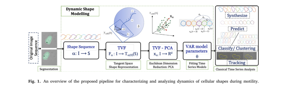
# The pipeline consists of the following steps:
# 1. Representing planar curves using the Square-Root Velocity Function (SRVF).
# 2. Computing Transported Velocity Fields (TVF) to represent shape dynamics.
# 3. Applying Principal Component Analysis (PCA) for dimensionality reduction (TVF-PCA).
# 4. Fitting a Vector Auto-Regressive (VAR) model to the low-dimensional time series.
# 5. Using VAR model parameters as features for classification.
#
# Required libraries:
# pip install numpy fdasrsf scikit-learn statsmodels matplotlib

import numpy as np
import fdasrsf as fs
from sklearn.decomposition import PCA
from sklearn.model_selection import train_test_split
from sklearn.svm import SVC
from sklearn.metrics import accuracy_score
from statsmodels.tsa.api import VAR
import matplotlib.pyplot as plt

def simulate_shape_data(num_sequences=40, seq_length=50, num_points=100, num_classes=4):
    """
    Simulates a dataset of shape sequences for demonstration purposes.
    The paper uses real microscopy data, but we'll generate synthetic data
    to make this code runnable.

    Args:
        num_sequences (int): Total number of sequences to generate.
        seq_length (int): The length of each shape time-series.
        num_points (int): The number of points discretizing each shape's boundary.
        num_classes (int): The number of distinct classes to simulate.

    Returns:
        tuple: A tuple containing:
            - all_sequences (list of np.ndarray): A list of shape sequences. Each sequence
              is a numpy array of shape (seq_length, num_points, 2).
            - labels (np.ndarray): An array of class labels for each sequence.
    """
    print("Simulating synthetic shape data...")
    all_sequences = []
    labels = []
    
    # Base shape (a circle)
    t = np.linspace(0, 2 * np.pi, num_points)
    base_shape = np.c_[np.cos(t), np.sin(t)]

    for i in range(num_sequences):
        class_id = i % num_classes
        sequence = []
        
        # Introduce class-specific deformations
        # This is a simplification. The paper uses a more complex simulation based on
        # Fourier coefficients of real data.
        freq1 = 2 + class_id
        freq2 = 3 + class_id
        
        current_shape = base_shape.copy()
        
        for j in range(seq_length):
            # Evolve the shape over time with some noise and class-specific patterns
            noise = np.random.randn(num_points, 2) * 0.02
            deformation = 0.1 * np.sin(t * freq1 + j * 0.1)[:, np.newaxis] * base_shape
            deformation += 0.08 * np.cos(t * freq2 + j * 0.15)[:, np.newaxis] * np.c_[-base_shape[:,1], base_shape[:,0]]
            
            current_shape += deformation * 0.1 + noise
            
            # Resample to maintain uniform point spacing
            resampled_shape = fs.resamplecurve(current_shape, num_points)
            sequence.append(resampled_shape)
            
        all_sequences.append(np.array(sequence))
        labels.append(class_id)
        
    print(f"Generated {num_sequences} sequences belonging to {num_classes} classes.")
    return all_sequences, np.array(labels)


def shapes_to_srvf(sequences):
    """
    Converts a list of shape sequences to their SRVF representation.

    Args:
        sequences (list): A list of shape sequences (np.ndarray).

    Returns:
        list: A list of SRVF sequences.
    """
    print("Converting shapes to SRVF representation...")
    srvf_sequences = []
    for seq in sequences:
        srvf_seq = []
        for shape in seq:
            # The fdasrsf library expects shape array of size (2, num_points)
            srvf = fs.curve_to_q(shape.T)
            srvf_seq.append(srvf.T) # Transpose back to (num_points, 2)
        srvf_sequences.append(np.array(srvf_seq))
    return srvf_sequences


def compute_tvf(srvf_sequences):
    """
    Computes the Transported Velocity Fields (TVF) for each SRVF sequence.
    This involves calculating shooting vectors and parallel transporting them.

    Args:
        srvf_sequences (list): A list of SRVF sequences.

    Returns:
        tuple: A tuple containing:
            - tvf_sequences (list): A list of TVF sequences.
            - initial_shapes_srvf (list): SRVFs of the first shape in each sequence.
    """
    print("Computing Transported Velocity Fields (TVF)...")
    tvf_sequences = []
    initial_shapes_srvf = [seq[0] for seq in srvf_sequences]

    for seq_idx, srvf_seq in enumerate(srvf_sequences):
        T = srvf_seq.shape[0]
        initial_srvf = initial_shapes_srvf[seq_idx].T # Shape (2, N) for fdasrsf
        
        tvf_seq = []
        
        # Path for parallel transport starts at the initial shape
        path = [initial_srvf]

        for t in range(T - 1):
            q1 = srvf_seq[t].T
            q2 = srvf_seq[t+1].T
            
            # Calculate shooting vector from q1 to q2
            # This is the initial velocity of the geodesic from q1 to q2
            geodesic_dist = fs.geod_dist(q1, q2)
            if np.isclose(geodesic_dist, 0):
                shooting_vector = np.zeros_like(q1)
            else:
                # Based on Eq. (1) in the paper
                shooting_vector = (geodesic_dist / np.sin(geodesic_dist)) * (q2 - np.cos(geodesic_dist) * q1)
            
            # Parallel transport the shooting vector from q1 back to the initial shape q0
            # The fdasrsf library provides parallel transport along a geodesic.
            # We approximate the path a(t) with a sequence of geodesics.
            path.append(q1)
            transported_vector = fs.parallel_transport(shooting_vector, q1, path[-2])
            
            # The paper transports along the entire path a(t) back to a(0).
            # We do this iteratively.
            current_transported_vector = transported_vector
            for i in range(len(path) - 2, 0, -1):
                current_transported_vector = fs.parallel_transport(current_transported_vector, path[i], path[i-1])

            tvf_seq.append(current_transported_vector.T.flatten())
        
        # Add a zero vector for the last time step as there is no alpha(T+1)
        tvf_seq.append(np.zeros_like(tvf_seq[-1]))
        tvf_sequences.append(np.array(tvf_seq))
        
    return tvf_sequences, initial_shapes_srvf


def tvf_pca_reduction(tvf_sequences, n_components=5):
    """
    Applies PCA to the pooled TVF data for dimensionality reduction.

    Args:
        tvf_sequences (list): List of TVF sequences.
        n_components (int): Number of principal components to keep.

    Returns:
        tuple: A tuple containing:
            - pca_sequences (list): List of low-dimensional time series.
            - pca_model (PCA): The fitted PCA model.
    """
    print(f"Performing PCA for dimensionality reduction (d={n_components})...")
    # Pool all TVF vectors from all sequences
    pooled_tvf = np.vstack(tvf_sequences)
    
    # Fit PCA on the pooled data
    pca = PCA(n_components=n_components)
    pca.fit(pooled_tvf)
    
    # Transform each sequence
    pca_sequences = [pca.transform(tvf_seq) for tvf_seq in tvf_sequences]
    
    return pca_sequences, pca


def fit_var_and_get_features(pca_sequences, maxlags=3):
    """
    Fits a VAR(p) model to each sequence and extracts parameters as features.

    Args:
        pca_sequences (list): List of low-dimensional time series.
        maxlags (int): The maximum lag order to consider for the VAR model.

    Returns:
        np.ndarray: An array of feature vectors, where each vector is the
                    flattened parameters of the fitted VAR model.
    """
    print("Fitting VAR models and extracting features...")
    features = []
    for seq in pca_sequences:
        # Select VAR model order (p) using an information criterion, e.g., BIC
        # For simplicity, as in the paper, we can test a few lags or use a fixed one.
        # Here we use a fixed lag for consistency.
        try:
            model = VAR(seq)
            # The paper uses BIC to select the best lag. For simplicity, we use a fixed lag.
            results = model.fit(maxlags=maxlags, ic='bic')
            
            # Extract parameters as features: coefficient matrices A_i and constant c
            var_params = results.params.flatten()
            features.append(var_params)
        except Exception as e:
            # Handle cases where VAR model fitting fails (e.g., short series)
            print(f"Warning: VAR model fitting failed for a sequence: {e}. Using zeros.")
            # Determine expected feature size from a successful fit
            d = pca_sequences[0].shape[1]
            p = maxlags
            expected_size = (1 + p * d) * d
            features.append(np.zeros(expected_size))

    # Pad features to have the same length (if different lags were used)
    max_len = max(len(f) for f in features)
    padded_features = np.array([np.pad(f, (0, max_len - len(f))) for f in features])
    
    return padded_features


def main():
    """
    Main function to run the entire pipeline.
    """
    # --- 1. Data Generation ---
    # In a real scenario, you would load your segmented cell contours here.
    # Each sequence would be a numpy array of shape (T, N, 2), where T is time,
    # N is number of points, and 2 is for (x, y) coordinates.
    all_sequences, labels = simulate_shape_data(num_sequences=50, seq_length=40, num_classes=4)

    # --- 2. Shape to SRVF Conversion ---
    srvf_sequences = shapes_to_srvf(all_sequences)

    # --- 3. Compute TVF ---
    # This is a complex step. The paper uses parallel transport along the path a.
    # The `fdasrsf` library's transport is along a geodesic between two points.
    # Our implementation is an approximation of the paper's method.
    tvf_sequences, _ = compute_tvf(srvf_sequences)

    # --- 4. TVF-PCA Dimensionality Reduction ---
    d = 5 # Number of principal components, as used in the paper
    pca_sequences, pca_model = tvf_pca_reduction(tvf_sequences, n_components=d)
    
    # --- 5. VAR Model Fitting and Feature Extraction ---
    # The paper explores different lags (p). We use a fixed lag for simplicity.
    var_features = fit_var_and_get_features(pca_sequences, maxlags=3)

    # --- 6. Classification ---
    print("Training and evaluating SVM classifier...")
    X_train, X_test, y_train, y_test = train_test_split(
        var_features, labels, test_size=0.3, random_state=42, stratify=labels
    )

    classifier = SVC(kernel='linear', C=1.0, random_state=42)
    classifier.fit(X_train, y_train)

    y_pred = classifier.predict(X_test)
    accuracy = accuracy_score(y_test, y_pred)

    print("\n--- Classification Results ---")
    print(f"Classifier: Support Vector Machine (SVM)")
    print(f"Features: Flattened VAR model parameters")
    print(f"Classification Accuracy: {accuracy:.4f}")

    # --- Visualization (Optional) ---
    # Plot one of the original and reconstructed sequences
    seq_to_plot_idx = 0
    original_seq = all_sequences[seq_to_plot_idx]
    
    # Reconstruct from PCA representation
    reconstructed_tvf = pca_model.inverse_transform(pca_sequences[seq_to_plot_idx])
    
    # Reconstruct shape sequence from TVF and initial shape
    # This is a complex inverse problem not fully detailed in this script.
    # For now, we just visualize the original data.
    fig, axes = plt.subplots(4, 10, figsize=(20, 8), sharex=True, sharey=True)
    fig.suptitle(f'Sample Simulated Shape Sequence (Class {labels[seq_to_plot_idx]})', fontsize=16)
    axes = axes.flatten()
    for i in range(min(40, len(original_seq))):
        ax = axes[i]
        shape = original_seq[i]
        ax.plot(shape[:, 0], shape[:, 1], c='b')
        ax.set_aspect('equal', 'box')
        ax.set_xticks([])
        ax.set_yticks([])
    for i in range(len(original_seq), len(axes)):
        axes[i].axis('off')
    plt.tight_layout(rect=[0, 0.03, 1, 0.95])
    plt.show()


if __name__ == '__main__':
    main()

References

- Deng, X., Sarkar, R., Labruyere, E., Olivo-Marin, J.-C., & Srivastava, A. (2026). Time-series analysis of cellular shapes using transported velocity fields. Pattern Recognition, 171, 112056.
- Srivastava, A., et al. (2011). Shape analysis of elastic curves in Euclidean spaces. IEEE TPAMI.
- Gordonov, S., et al. (2016). Time series modeling of live-cell shape dynamics. Integrative Biology.
Related posts, You May like to read
- 7 Shocking Truths About Knowledge Distillation: The Good, The Bad, and The Breakthrough (SAKD)
- 7 Revolutionary Breakthroughs in Medical Image Translation (And 1 Fatal Flaw That Could Derail Your AI Model)
- 7 Revolutionary Brain Disease Prediction: How AI Beats Disease (But One Flaw Remains)
- 1 Revolutionary Breakthrough in AI Object Detection: GridCLIP vs. Two-Stage Models