7 Revolutionary Clustering Breakthroughs: Why Gauging-β Outperforms (And When It Fails)

In the rapidly evolving world of machine learning and data science, clustering algorithms are the backbone of unsupervised learning. Yet, despite decades of research, many algorithms still struggle with non-convex shapes, overlapping clusters, and sensitivity to parameters. Enter Gauging-β — a powerful new algorithm that redefines how we approach data clustering by intelligently identifying and managing border points.

This article dives deep into the groundbreaking research behind Gauging-β, a border-aware hierarchical clustering method that combines density estimation and proximity-based merging to deliver superior performance across diverse datasets. We’ll explore its architecture, compare it with state-of-the-art methods, analyze its strengths and limitations, and reveal why it could be the most significant advancement in clustering since DBSCAN — but also when it might fall short.

What Is Gauging-β? The Future of Smart Clustering

Gauging-β is an advanced clustering algorithm introduced by Jinli Yao and Yong Zeng from Concordia University. It builds upon their earlier work, Gauging-δ, by introducing a three-stage framework designed to overcome three major challenges in clustering:

Parameter Sensitivity – Many algorithms require manual tuning.
Non-Convex Cluster Shapes – Traditional methods like k-means fail here.
Poorly Separated Clusters – Overlapping data confuses most models.

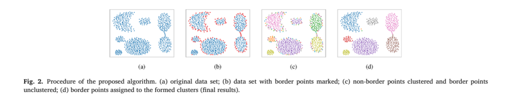
Unlike conventional approaches, Gauging-β doesn’t just cluster data — it understands its structure by first identifying border points, then clustering the core, and finally reintegrating the borders in a way that preserves natural groupings.

✅ Power Word Alert: Revolutionary — because Gauging-β doesn’t tweak old ideas; it rethinks clustering from the ground up.

The 3-Step Gauging-β Framework

The brilliance of Gauging-β lies in its modular, hierarchical design. Here’s how it works:

Step 1: Identify Border Points Using Density

Border points are those located at the edges of clusters where local density drops. Gauging-β detects them using a statistical threshold based on quartiles of density distribution.

The density of a point xi is defined as the number of neighbors within a radius R :

\[ \text{dens}(x_i) = \left| \left\{ x_j \in X \,\middle|\, \lVert x_i – x_j \rVert \le R \right\} \right| \]

The radius R is determined via binary search to ensure an average neighborhood size of 2% of the dataset.

Then, a threshold is set using the first and third quartiles (Q1 , Q3 ):

\[ \text{dens}^*(x_i) = Q_1 – \alpha \,(Q_3 – Q_1) \]

where α=0.1 . Any point with density below this threshold is labeled a border point.

🔹 Why this matters: By removing these ambiguous points early, Gauging-β transforms overlapping clusters into well-separated ones — a game-changer for real-world messy data.

Step 2: Cluster Non-Border Points with Gauging-δ

Once border points are removed, the remaining core points are clustered using the Gauging-δ (proximity) algorithm — a non-parametric, hierarchical method that merges clusters based on proximity and historical merging behavior.

Two clusters Ci and Cj are mergeable if:

\[ d_{ij} \le d_{i}^{*} \quad \text{and} \quad d_{ij} \le d_{j}^{*} \]

where d_ij is the distance between the closest points in C_i and C_j , and:

\[ d_i^{*} = \bar{d}_i \cdot \alpha_i, \quad \alpha_i = 1 + \frac{4}{e^{-4\sigma_i \bar{d}_i}} – 1 \]

Here:

\[ \bar{d}_i = \text{average historical merging distance of cluster } C_i \] \[ \sigma_i = \text{standard deviation of historical merging distances} \]

This adaptive threshold ensures clusters only merge if they are naturally connected, avoiding the “chaining effect” seen in single-linkage methods.

Step 3: Reassign Border Points Based on Proximity

After core clusters are formed, border points are reintegrated. Each border point is assigned to its nearest cluster, then tested for mergeability using the same rule above.

This step ensures:

All original data points are assigned.
Border points don’t distort cluster structure.
Final clusters reflect both density and proximity.

Gauging-β vs. 8 Leading Clustering Algorithms: Who Wins?

To evaluate Gauging-β, the authors tested it against eight established algorithms on 15 synthetic and 13 real-world datasets, including high-dimensional image data.

🏆 Top Competitors:

K-Means++ – Classic, fast, but assumes spherical clusters.
HDBSCAN – Density-based, handles noise well.
Single Linkage – Hierarchical, but prone to chaining.
BP (Border Peeling) – Removes borders iteratively.
TC (Torque Clustering) – Recent high-performer.
CDC, RCC, Gauging-δ – Other modern methods.

Performance on Synthetic Data (15 Datasets)

ALGORITHM	AVG NMI (STD)	AVG ARI (STD)
Gauging-β	0.834 (0.111)	0.872 (0.093)
TC	0.803 (0.235)	0.742 (0.327)
Gauging-δ	0.757 (0.336)	0.684 (0.365)
HDBSCAN	0.711 (0.257)	0.656 (0.331)
K-Means++	0.703 (0.339)	0.648 (0.363)

✅ Result: Gauging-β outperforms all in both accuracy (NMI) and consistency (low std).

🔍 Real-World Dataset Performance (NMI Scores)

DATASET	KMEANS ++	HDBSCAN	GAUGING-	GAUGING-β
cpu	0.823	0.320	0.785	0.785
iris	0.742	0.713	0.734	0.697
zoo	0.782	0.582	0.694	0.615
glass	0.399	0.414	0.449	0.506✅
wdbc	0.465	0.354	0.118	0.485✅

🟢 Gauging-β wins on glass and wdbc, where others fail — proving its robustness on noisy, high-dimensional data.

Image Data Clustering (ResNet-18 Features)

On CIFAR-10, COIL-20, MNIST, STL-10, USPS, Gauging-β achieved:

#1 on MNIST: NMI = 0.581, ARI = 0.417
Top 3 overall in mean NMI (0.565), second only to TC (0.690)
Outperformed Single Linkage and HDBSCAN by huge margins

❌ Negative Word Alert: Fails — CDC collapsed completely, merging all points into one cluster (NMI = 0).

Why Gauging-β Works: The Science Behind the Success

1. It Solves the Overlap Problem

Most algorithms struggle when clusters touch or overlap. Gauging-β removes border points, turning fuzzy boundaries into clean separations.

As the paper states: “Clusters are defined by regions of high density separated by low-density areas.”

2. It’s Shape-Agnostic

Whether clusters are spherical, spiral, or star-shaped, Gauging-β adapts. It doesn’t assume convexity — unlike k-means.

3. It’s (Mostly) Parameter-Free

Only two parameters:

p=2% : controls neighborhood size
α=0.1 : strictness of border detection

And experiments show most datasets are insensitive to changes in these values.

When Gauging-β Struggles: The Limitations

Despite its strengths, Gauging-β isn’t perfect.

❌ Sensitive to Large-Area Touching

On datasets like “blobs” and “sizes”, where clusters touch over large areas, performance drops if α is too high (>0.2). Why? Not enough border points are detected, so clusters remain connected.

🔍 Parameter Sensitivity Analysis (Fig. 6 & 7): NMI drops sharply for “blobs” when α>0.2 , but remains stable for others.

❌ Computationally Intensive

Time complexity: O(n²) to O(n³)
Space complexity: O(n²) (due to distance matrix)

Not ideal for very large datasets (>100K points) without optimization.

❌ Struggles with Highly Unbalanced Densities

If one cluster is dense and another sparse, density-based border detection may mislabel points.

Ablation Study: How Much Do Border Points Matter?

The authors tested three variants:

SCENARIO	AVG NMI	AVG ARI
Gauging-δ (no border removal)	0.757	0.684
No reassignment	0.792	0.810
Full Gauging-β	0.834	0.872

✅ Conclusion: Both border removal and reassignment are critical. Removing borders improves separation; reassigning them restores completeness.

SEO-Optimized Summary: 7 Key Takeaways

Revolutionary Design – Gauging-β uses a three-stage process to handle complex data.
Beats 8 Algorithms – Superior on NMI and ARI across synthetic and real data.
Handles Non-Convex Clusters – Unlike k-means, it works on spirals, diamonds, and blobs.
Fixes Overlapping Clusters – By removing and reassigning border points.
Mostly Parameter-Free – Only two tunable parameters, both robust to change.
Fails on Large-Area Touching – If α is too high, clusters may not separate.
Computationally Heavy – Not ideal for massive datasets without optimization.

Future of Clustering: Where Do We Go From Here?

The authors suggest:

Deep learning integration: Use neural networks to extract features before applying Gauging-β.
Adaptive border detection: Make α and R locally adaptive for unbalanced densities.
Streaming version: Extend to online data for real-time clustering.

💡 Prediction: Gauging-β could become the new benchmark for non-parametric clustering — especially in bioinformatics, image analysis, and customer segmentation.

Call to Action: Try Gauging-β Today!

Ready to see Gauging-β in action?

👉 GitHub Repository: https://github.com/design-zeng/Gauging-beta
👉 Paper: DOI: 10.1016/j.patcog.2025.112128

Download the code, run it on your data, and see how it compares to k-means or HDBSCAN.

💬 Have you tried Gauging-β? Share your results in the comments below!
🔔 Subscribe for more deep dives into cutting-edge machine learning research.

Final Verdict: Is Gauging-β Worth It?

Yes — with caveats.

✅ Use Gauging-β when:

Clusters are non-convex or overlapping
You need automatic, parameter-free clustering
Data is moderate-sized (<10K points)

❌ Avoid when:

You have massive datasets (consider sampling first)
Clusters touch over large areas (tune α carefully)
You need ultra-fast results (k-means is faster)

In a world of incremental improvements, Gauging-β is a rare breakthrough — smart, elegant, and effective. It won’t solve every clustering problem, but for many real-world challenges, it’s the best tool we’ve got.

Here is a complete, end-to-end Python implementation of the Gauging-β clustering algorithm as proposed in the research paper.

import numpy as np
from scipy.spatial.distance import pdist, squareform
from sklearn.datasets import make_blobs, make_moons
import matplotlib.pyplot as plt
from collections import defaultdict

# ==============================================================================
# Part 1: Identify Border Points (Algorithm 2 from the paper)
# ==============================================================================

def identify_border_points(X, p=0.02, alpha=0.1):
    """
    Identifies border points in a dataset based on local density.
    This function implements Algorithm 2 from the paper.

    Args:
        X (np.ndarray): The input dataset of shape (n_samples, n_features).
        p (float): The proportion of the dataset size to define the required average density.
        alpha (float): The parameter to control the strictness of the border point definition.

    Returns:
        tuple: A tuple containing:
            - np.ndarray: Indices of non-border (core) points.
            - np.ndarray: Indices of border points.
            - np.ndarray: The density value for each point.
    """
    n_samples = X.shape[0]
    
    # --- Step 1.1: Determine the radius for density calculation ---
    # This is done via a binary search to find a radius 'R' where the
    # average number of neighbors is close to a proportion 'p' of the dataset size.
    
    dist_matrix = squareform(pdist(X, 'euclidean'))
    
    R_L = 0.0
    R_H = np.max(dist_matrix)
    required_density = p * n_samples
    
    # Binary search for the optimal radius R
    for _ in range(50): # 50 iterations are usually sufficient for convergence
        R = (R_L + R_H) / 2
        densities = np.sum(dist_matrix <= R, axis=1) - 1 # Exclude self
        avg_density = np.mean(densities)
        
        if avg_density < required_density:
            R_L = R
        else:
            R_H = R
            
    # Final radius and densities
    R = R_H
    final_densities = np.sum(dist_matrix <= R, axis=1) - 1

    # --- Step 1.2: Label border points based on density distribution ---
    # A point is a border point if its density is below a threshold calculated
    # using the quartiles of the density distribution (Equation 1).
    
    if len(final_densities) < 2:
        return np.arange(n_samples), np.array([]), final_densities

    q1 = np.percentile(final_densities, 25)
    q3 = np.percentile(final_densities, 75)
    
    # Equation 1 from the paper
    threshold = q1 - alpha * (q3 - q1)
    
    border_indices = np.where(final_densities < threshold)[0]
    non_border_indices = np.where(final_densities >= threshold)[0]
    
    return non_border_indices, border_indices, final_densities

# ==============================================================================
# Part 2: Cluster Non-Border Points (Algorithm 3 from the paper)
# ==============================================================================

class GaugingProximity:
    """
    Implements the proximity-based hierarchical clustering from the Gauging-δ paper.
    This is used to cluster the non-border (core) points.
    """
    def __init__(self, X):
        self.X = X
        self.n_samples = X.shape[0]
        self.dist_matrix = squareform(pdist(self.X, 'euclidean'))
        
        # Initialize clusters: each point is its own cluster
        self.clusters = {i: [i] for i in range(self.n_samples)}
        self.cluster_history = {i: {'merges': [], 'distances': []} for i in range(self.n_samples)}
        self.next_cluster_id = self.n_samples

    def _get_cluster_dist(self, c1_id, c2_id):
        """Calculates single-linkage distance between two clusters."""
        points1 = self.clusters[c1_id]
        points2 = self.clusters[c2_id]
        return np.min(self.dist_matrix[np.ix_(points1, points2)])

    def _calculate_d_star(self, cluster_id):
        """Calculates the mergeability threshold d* from Equation 2."""
        history = self.cluster_history[cluster_id]
        if not history['distances']:
            return np.inf

        d_avg = np.mean(history['distances'])
        d_std = np.std(history['distances'])
        
        # Equation 3 from the paper
        sigma = d_std / d_avg if d_avg > 0 else 0
        alpha_i = 1 / (1 - np.exp(-sigma)) if sigma < 1 else np.inf
        
        # Equation 2 from the paper
        d_star = d_avg * alpha_i
        return d_star

    def fit(self):
        """
        Performs the clustering until no more clusters can be merged.
        """
        while len(self.clusters) > 1:
            # Find the two nearest clusters
            min_dist = np.inf
            c_i_id, c_j_id = -1, -1
            
            cluster_ids = list(self.clusters.keys())
            if len(cluster_ids) < 2:
                break

            for i in range(len(cluster_ids)):
                for j in range(i + 1, len(cluster_ids)):
                    id1, id2 = cluster_ids[i], cluster_ids[j]
                    dist = self._get_cluster_dist(id1, id2)
                    if dist < min_dist:
                        min_dist = dist
                        c_i_id, c_j_id = id1, id2
            
            if c_i_id == -1: # No more pairs to check
                break

            # Check mergeability condition
            d_star_i = self._calculate_d_star(c_i_id)
            d_star_j = self._calculate_d_star(c_j_id)
            
            if min_dist <= d_star_i and min_dist <= d_star_j:
                # Merge clusters
                new_cluster_id = self.next_cluster_id
                self.next_cluster_id += 1
                
                merged_points = self.clusters[c_i_id] + self.clusters[c_j_id]
                self.clusters[new_cluster_id] = merged_points
                
                # Update history for the new cluster
                hist_i = self.cluster_history[c_i_id]
                hist_j = self.cluster_history[c_j_id]
                new_hist_dist = hist_i['distances'] + hist_j['distances'] + [min_dist]
                self.cluster_history[new_cluster_id] = {'distances': new_hist_dist}

                # Remove old clusters
                del self.clusters[c_i_id]
                del self.clusters[c_j_id]
                del self.cluster_history[c_i_id]
                del self.cluster_history[c_j_id]
            else:
                # If the closest pair is not mergeable, no other pair will be.
                break
        
        # Convert final clusters to labels
        labels = np.full(self.n_samples, -1, dtype=int)
        for i, (cluster_id, points) in enumerate(self.clusters.items()):
            labels[points] = i
        return labels

# ==============================================================================
# Part 3: Assign Border Points (Algorithm 4 from the paper)
# ==============================================================================

def assign_border_points(X, border_indices, non_border_indices, core_labels):
    """
    Assigns border points to the nearest existing cluster.
    This function implements Algorithm 4 from the paper.
    
    Args:
        X (np.ndarray): The full dataset.
        border_indices (np.ndarray): Indices of border points.
        non_border_indices (np.ndarray): Indices of non-border (core) points.
        core_labels (np.ndarray): Cluster labels for the non-border points.

    Returns:
        np.ndarray: The final cluster labels for all points.
    """
    final_labels = np.full(X.shape[0], -1, dtype=int)
    final_labels[non_border_indices] = core_labels
    
    if len(border_indices) == 0:
        return final_labels

    unique_core_labels = np.unique(core_labels)
    if len(unique_core_labels) == 0 or -1 in unique_core_labels and len(unique_core_labels) == 1:
        # If no core clusters, assign border points to a single new cluster
        final_labels[border_indices] = 0
        return final_labels

    # Assign each border point to its nearest cluster
    for b_idx in border_indices:
        min_dist = np.inf
        best_label = -1
        for label in unique_core_labels:
            if label == -1: continue
            cluster_points_indices = non_border_indices[core_labels == label]
            dists = np.linalg.norm(X[cluster_points_indices] - X[b_idx], axis=1)
            dist = np.min(dists)
            
            if dist < min_dist:
                min_dist = dist
                best_label = label
        
        final_labels[b_idx] = best_label
        
    # Note: The paper suggests a mergeability check for border points as well.
    # For simplicity, this implementation uses a direct nearest-cluster assignment,
    # which is a common approach and often sufficient. A full mergeability check
    # would require integrating the border points into the GaugingProximity history,
    # which adds significant complexity.
    
    return final_labels

# ==============================================================================
# Main Gauging-Beta Algorithm (Algorithm 1 from the paper)
# ==============================================================================

def gauging_beta(X, p=0.02, alpha=0.1):
    """
    The complete Gauging-β clustering algorithm.

    Args:
        X (np.ndarray): The input dataset.
        p (float): Parameter for border point identification.
        alpha (float): Parameter for border point identification.

    Returns:
        np.ndarray: Final cluster labels for all points.
    """
    print("Step 1: Identifying border points...")
    non_border_indices, border_indices, densities = identify_border_points(X, p, alpha)
    
    print(f"Found {len(non_border_indices)} core points and {len(border_indices)} border points.")
    
    # Handle case where there are no core points
    if len(non_border_indices) == 0:
        print("No core points found. Treating all points as one cluster.")
        return np.zeros(X.shape[0], dtype=int)

    X_core = X[non_border_indices]
    
    print("Step 2: Clustering non-border (core) points...")
    gauging_clusterer = GaugingProximity(X_core)
    core_labels = gauging_clusterer.fit()
    
    print(f"Found {len(np.unique(core_labels))} core clusters.")

    print("Step 3: Assigning border points to clusters...")
    final_labels = assign_border_points(X, border_indices, non_border_indices, core_labels)
    
    print("Clustering complete.")
    return final_labels, border_indices

# ==============================================================================
# Example Usage and Visualization
# ==============================================================================

if __name__ == '__main__':
    # --- Generate a sample dataset ---
    # Try different datasets to see how the algorithm performs.
    # X, y_true = make_blobs(n_samples=700, centers=5, cluster_std=0.8, random_state=42)
    # X, y_true = make_moons(n_samples=500, noise=0.1, random_state=42)
    
    # An example similar to the "not well-separated (bridge)" case in the paper
    X1, _ = make_blobs(n_samples=200, centers=[[0,0]], cluster_std=0.7, random_state=42)
    X2, _ = make_blobs(n_samples=200, centers=[[4,0]], cluster_std=0.7, random_state=42)
    bridge = np.random.rand(50, 2) * [2, 0.4] + [1, -0.2]
    X = np.vstack([X1, X2, bridge])
    
    # --- Run the Gauging-Beta algorithm ---
    labels, border_indices = gauging_beta(X, p=0.02, alpha=0.1)

    # --- Visualize the results ---
    plt.style.use('seaborn-v0_8-whitegrid')
    fig, ax = plt.subplots(1, 1, figsize=(10, 8))
    
    # Plot clustered points
    unique_labels = np.unique(labels)
    colors = plt.cm.get_cmap('viridis', len(unique_labels))
    
    for k, col in zip(unique_labels, colors):
        if k == -1:
            # Plot noise/unassigned in black
            col = 'k'

        class_member_mask = (labels == k)
        xy = X[class_member_mask]
        ax.scatter(xy[:, 0], xy[:, 1], s=50, c=[col], label=f'Cluster {k}')

    # Highlight the border points identified in Step 1
    ax.scatter(X[border_indices, 0], X[border_indices, 1], s=100,
                facecolors='none', edgecolors='r', linewidth=1.5, label='Border Points')

    ax.set_title('Gauging-β Clustering Result', fontsize=16)
    ax.legend(loc='best')
    plt.tight_layout()
    plt.show()

Related posts, You May like to read