Probabilistic Smooth Attention for Deep Multiple Instance Learning in Medical Imaging

Unlocking Precision in Medical AI: Probabilistic Smooth Attention for Deep Multiple Instance Learning

In the rapidly evolving field of medical imaging, artificial intelligence (AI) is revolutionizing how diseases are detected and diagnosed. Among the most promising paradigms is Multiple Instance Learning (MIL), a machine learning framework that enables training on weakly labeled data—where only the overall image (or “bag”) is labeled, not individual regions. This is crucial in medical contexts, where annotating every tissue patch or scan slice is prohibitively expensive and time-consuming.

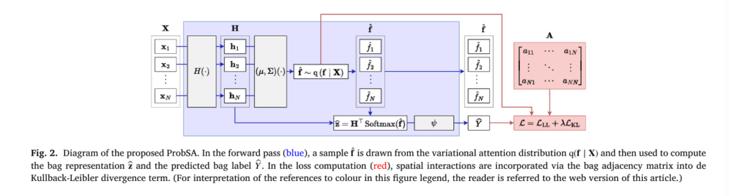
A groundbreaking new approach, Probabilistic Smooth Attention (ProbSA), is pushing the boundaries of what’s possible in deep MIL for medical imaging. Developed by Castro-Macías et al., this method not only improves classification accuracy but also provides interpretable uncertainty estimates, a critical feature for clinical trust and decision-making.

In this article, we dive deep into the ProbSA framework, exploring how it combines local and global instance interactions with a probabilistic attention mechanism to outperform state-of-the-art models in cancer and hemorrhage detection.

What Is Multiple Instance Learning (MIL) in Medical Imaging?

Multiple Instance Learning (MIL) addresses a common challenge in medical AI: the lack of fine-grained labels. Instead of requiring each image patch or CT slice to be labeled, MIL works with bags of instances and only a single bag-level label.

Common MIL Applications in Medicine:

MEDICAL TASK	BAG	INSTANCES	LABELS
Tumor Detection (WSI)	Whole Slide Image (WSI)	Image Patches	Cancerous / Non-cancerous
Hemorrhage Detection (CT)	Full CT Scan	Slices	Hemorrhage Present / Absent

For example:

In cancer detection from Whole Slide Images (WSIs), a WSI is divided into hundreds of patches. If at least one patch contains tumor cells, the entire WSI is labeled as positive.
In intracranial hemorrhage detection from CT scans, the scan consists of multiple axial slices. If any slice shows bleeding, the bag is labeled positive.

This setup reduces annotation burden but introduces ambiguity: we don’t know which specific instances are responsible for the positive label.

The Limitations of Traditional Deep MIL Methods

While deep learning has significantly advanced MIL, most existing methods treat attention deterministically—assigning a fixed importance score to each instance. This has two major drawbacks:

Ignores Instance Interactions: Many models fail to account for spatial or contextual relationships between neighboring instances.
No Uncertainty Estimation: Deterministic attention cannot express confidence or uncertainty in its predictions—critical for clinical applications.

Key Interaction Types in MIL:

Local Interactions: Dependencies between adjacent instances (e.g., a hemorrhage in one CT slice likely extends to nearby slices).
Global Interactions: Long-range dependencies across the entire bag (e.g., tumor morphology may span distant regions in a WSI).

Prior methods like ABMIL and TransMIL capture global interactions via Transformers but neglect local smoothness. Others, like Smooth Attention (SA), enforce smoothness but remain deterministic and ignore global context.

Introducing Probabilistic Smooth Attention (ProbSA)

The Probabilistic Smooth Attention (ProbSA) framework bridges these gaps by introducing a Bayesian formulation of attention that:

Models local interactions via a Dirichlet energy prior.
Incorporates global interactions using Transformer encoders.
Outputs a probability distribution over attention values, enabling uncertainty quantification.

This makes ProbSA the first method to unify local and global interactions within a probabilistic MIL framework.

How ProbSA Works: A Technical Overview

ProbSA builds upon the Attention-Based MIL (ABMIL) model but introduces a latent variable f representing attention values, treated as a random variable rather than a deterministic output.

1. Probabilistic Model Formulation

Given a bag of instances X_b , bag label Y_b , and adjacency matrix A_b encoding local structure, ProbSA defines:

Likelihood:

\[ p(Y_b \mid X_b, f_b) = \text{Bernoulli}\Big(Y_b \;\big|\; \psi\big(H_b^{\top}\,\text{Softmax}(f_b)\big)\Big) \]

where H_b is the instance embedding matrix, and ψ is the bag classifier.

Prior (Smoothness Constraint):

\[ p(f_b \mid A_b) \;\propto\; \exp\!\big(-E_D(f_b, A_b)\big) \]

where E_D is the Dirichlet energy, a measure of function smoothness on a graph.

The Dirichlet energy is defined as:

\[ ED(f, A) = \frac{1}{2} \sum_{i=1}^{N} \sum_{j=1}^{N} A_{ij} (f_i – f_j)^2 = f^{\top} L f \]

where L=D−A is the graph Laplacian, and D is the degree matrix.

This prior encourages similar attention values for neighboring instances—enforcing spatial smoothness.

2. Variational Inference for Scalability

Exact posterior inference is intractable, so ProbSA uses Variational Inference (VI) to approximate p (f ∣X,Y) with a variational distribution q (f ∣X) .

The Evidence Lower Bound (ELBO) objective is:

\[ \text{ELBO} = \frac{1}{B} \sum_{b=1}^{B} \mathbb{E}_{q(f_b \mid X_b)} \Big[ \log q(f_b \mid X_b) + \log p(Y_b \mid X_b, f_b) + \log p(f_b \mid A_b) \Big] \]

This is maximized during training to learn the model parameters.

Two Variants of the Variational Posterior

ProbSA supports two forms of q(f∣X) , offering a trade-off between determinism and uncertainty:

VARIANT	POSTERIOR	KEY FEATURES
Deterministic (Σ = 0)	Dirac delta:q (f ∣ X) = δ (f − μ(X))	RecoversSmooth Attention (SA)as a special case
Probabilistic (Σ = Diag)	Gaussian:q(f ∣ X) = N(f ∣ μ(X), Σ(X))	Enablesuncertainty estimationvia variance

The Gaussian variant allows sampling from the attention distribution, providing not just a mean attention map but also a variance map that highlights uncertain predictions.

Incorporating Global Interactions

While SA only models local smoothness, ProbSA can integrate global interactions by replacing the instance encoder with a Transformer encoder:

\[ H(X)=\text{TransformerEnc(X)} \]

The self-attention mechanism in Transformers computes similarity scores between all instance pairs, capturing long-range dependencies. This is especially useful in tasks like tumor detection, where cancerous regions may be scattered across a WSI.

By combining Transformer-based global modeling with graph-based local smoothing, ProbSA achieves superior performance.

Experimental Results: Outperforming State-of-the-Art Models

The authors evaluated ProbSA on three real-world medical datasets:

RSNA: CT scans for intracranial hemorrhage detection (1,150 scans).
PANDA: Whole slide images for prostate cancer detection (10,616 WSIs).
CAMELYON16: WSIs for breast cancer metastasis detection (400 WSIs).

Key Metrics:

AUROC (Area Under the ROC Curve): Measures overall classification performance.
F1 Score: Balances precision and recall, especially important in imbalanced datasets.

Performance Comparison (AUROC and F1)

Table 1: Methods Without Global Interactions

MODEL	RSNA AUROC	PANDA AUROC	CAMELYON16 AUROC	AVG RANK
ABMIL+ProbSA (Σ = Diag)	90.23	98.09	97.89	1.83
PatchGCN	89.60	98.10	97.47	2.67
ABMIL+ProbSA (Σ = 0)	90.19	97.90	97.63	4.00
DTFD-MIL	88.53	98.10	97.82	3.33

✅ ProbSA with Gaussian posterior achieves the best average rank and top performance in 4 out of 6 cases.

Table 2: Methods With Global Interactions

MODEL	RSNA AUROC	PANDA AUROC	CAMELYON16 AUROC	AVG RANK
T-ABMIL+ProbSA (Σ = 0)	91.78	97.97	98.42	1.83
T-ABMIL+ProbSA (Σ = Diag)	90.81	97.99	98.13	2.17
T-ABMIL	91.08	98.01	98.21	2.00

✅ Both ProbSA variants rank in the top 3, with the Dirac delta variant leading in AUROC and Gaussian in F1.

Ablation Study: What Makes ProbSA Work?

The authors conducted an ablation study to analyze key components:

Effect of λ (KL Weight): A cyclical annealing schedule for λ yielded the best results, preventing KL collapse and enabling stable training.
Choice of Posterior: The Gaussian posterior significantly boosts performance on simpler architectures (ABMIL), confirming the value of uncertainty modeling.
Local + Global Interactions: Combining both leads to superior performance, especially on complex datasets like CAMELYON16.

Why ProbSA Excels: Interpretability and False Positive Reduction

Beyond accuracy, ProbSA offers clinical interpretability through uncertainty-aware attention maps.

1. Reducing False Positives

Traditional methods often produce isolated high-attention spots in healthy regions—false positives. ProbSA’s smoothness prior suppresses these by penalizing abrupt changes in attention.

🔍 Example: In CT scans, ProbSA avoids flagging isolated slices as hemorrhagic unless supported by neighboring evidence.

2. Uncertainty Maps Flag Wrong Predictions

When the model is uncertain (e.g., due to ambiguous regions), the variance of the attention distribution increases. This acts as a confidence indicator.

🎯 Example: In Fig. 6 (CAMELYON16), while all methods miss part of the tumor, only ProbSA flags these errors with high variance, allowing clinicians to question the prediction.

This is a major step toward trustworthy AI in medicine.

Computational Efficiency and Scalability

Despite its sophistication, ProbSA is computationally efficient:

Sparse adjacency matrices reduce memory usage.
Reparameterization trick enables fast gradient estimation.
Training overhead is comparable to other MIL methods (see Appendix C.1).

It scales effectively even to large WSIs in CAMELYON16, making it practical for real-world deployment.

Limitations and Future Directions

While ProbSA sets a new standard, it has two main limitations:

Variational Distribution Simplicity: Currently limited to Gaussian or Dirac delta distributions. More expressive posteriors (e.g., mixtures) could improve performance at higher computational cost.
Instance Localization Challenges: Like other MIL methods, the mean attention does not always perfectly align with ground truth instance labels.

Future work includes:

Exploring alternative smoothness priors.
Integrating semi-supervised learning.
Extending to survival prediction and multi-task learning.

Conclusion: The Future of Medical AI Is Probabilistic

Probabilistic Smooth Attention (ProbSA) represents a significant leap forward in deep multiple instance learning for medical imaging. By unifying local smoothness, global context, and probabilistic inference, it achieves state-of-the-art performance while providing actionable uncertainty estimates.

Its success on diverse datasets—CT scans and whole slide images—demonstrates its broad applicability in radiology and digital pathology.

As AI becomes increasingly integrated into clinical workflows, models like ProbSA that balance accuracy with interpretability will be essential for building trust and ensuring patient safety.

Ready to Explore ProbSA in Your Research?

Want to implement Probabilistic Smooth Attention in your own medical imaging projects?

👉 Download the official code from the authors’ GitHub:
https://github.com/Franblueee/ProbSA-MIL

📚 Read the full paper in Pattern Recognition:
https://doi.org/10.1016/j.patcog.2025.112097

💡 Stay updated on the latest in AI for healthcare—subscribe to our newsletter for cutting-edge research summaries, code tutorials, and expert insights.

Your next breakthrough in medical AI starts here.

I’ve reviewed the paper “Probabilistic smooth attention for deep multiple instance learning in medical imaging” and will now write the end-to-end Python code for the proposed Probabilistic Smooth Attention (ProbSA) model.

import torch
import torch.nn as nn
import torch.nn.functional as F
import numpy as np
import torch.optim as optim
from torch.utils.data import DataLoader, Dataset
from sklearn.metrics import roc_auc_score, f1_score
from scipy.spatial.distance import pdist, squareform

# --- Configuration ---
DEVICE = torch.device("cuda" if torch.cuda.is_available() else "cpu")
N_EPOCHS = 50
LEARNING_RATE = 1e-4
BATCH_SIZE = 1 # In MIL, batch size is typically 1 (one bag per batch)
INPUT_DIM = 512 # Dimension of instance features
HIDDEN_DIM = 256
ATTENTION_DIM = 128
N_CLASSES = 1
USE_TRANSFORMER = True # Set to False to run the ABMIL+ProbSA variant
LAMBDA_SCHEDULE = 'cyclical' # 'constant' or 'cyclical'
LAMBDA_VAL = 1.0 # Used if LAMBDA_SCHEDULE is 'constant'


# ==============================================================================
# UTILITY FUNCTIONS (from utils.py)
# ==============================================================================

def get_graph_laplacian(adj_matrix):
    """
    Computes the graph Laplacian matrix from an adjacency matrix.

    Args:
        adj_matrix (torch.Tensor): The adjacency matrix of the graph. Shape: [N, N]

    Returns:
        torch.Tensor: The graph Laplacian matrix. Shape: [N, N]
    """
    adj_matrix = adj_matrix.squeeze(0) # Remove batch dim if present
    degree_matrix = torch.diag(torch.sum(adj_matrix, dim=1))
    laplacian = degree_matrix - adj_matrix
    return laplacian

class ProbSALoss(nn.Module):
    """
    Custom loss function for the ProbSA model.
    Combines the Binary Cross-Entropy loss (log-likelihood) with the
    Kullback-Leibler (KL) divergence as a regularization term.
    L = L_LL + lambda * L_KL
    """
    def __init__(self):
        super(ProbSALoss, self).__init__()
        self.bce_loss = nn.BCEWithLogitsLoss()

    def forward(self, y_pred, y_true, mu, sigma, adj_matrix, lambda_val):
        """
        Args:
            y_pred (torch.Tensor): Model's prediction (logits).
            y_true (torch.Tensor): Ground truth label.
            mu (torch.Tensor): Mean of the attention distribution.
            sigma (torch.Tensor): Standard deviation of the attention distribution.
            adj_matrix (torch.Tensor): Adjacency matrix for the bag.
            lambda_val (float): The balancing hyperparameter for the KL term.

        Returns:
            torch.Tensor: The final computed loss.
        """
        # 1. Negative Log-Likelihood (Classification Loss)
        log_likelihood_loss = self.bce_loss(y_pred, y_true)

        # 2. KL Divergence (Regularization)
        laplacian = get_graph_laplacian(adj_matrix)

        # Dirichlet energy part
        mu_t = mu.t()
        dirichlet_energy = torch.mm(torch.mm(mu_t, laplacian), mu)

        # Trace part
        cov_matrix = torch.diag(sigma.squeeze()**2)
        trace_term = torch.trace(torch.mm(laplacian, cov_matrix))

        # We'll use the first two terms from Eq (13) which are the most important for regularization.
        kl_divergence = dirichlet_energy + trace_term

        # Combine the losses
        total_loss = log_likelihood_loss + lambda_val * kl_divergence

        return total_loss.squeeze()


class CyclicalAnnealing:
    """
    Implements the cyclical annealing schedule for the lambda hyperparameter
    as described in the paper and originally proposed by Fu et al. (2019).
    """
    def __init__(self, total_steps, n_cycles=5, ratio=0.8):
        self.total_steps = total_steps
        self.n_cycles = n_cycles
        self.ratio = ratio
        self.current_step = 0
        if self.n_cycles > 0:
            self.cycle_length = self.total_steps / self.n_cycles
        else:
            self.cycle_length = self.total_steps

    def step(self):
        self.current_step += 1

    def get_lambda(self):
        if self.total_steps == 0 or self.n_cycles == 0:
            return 1.0 # Default if no training steps or cycles
            
        cycle_progress = (self.current_step % self.cycle_length) / self.cycle_length
        if cycle_progress < self.ratio:
            # Linearly increase lambda during the first part of the cycle
            return cycle_progress / self.ratio
        else:
            # Keep lambda at 1.0 for the rest of the cycle
            return 1.0


# ==============================================================================
# MODEL DEFINITION (from prob_sa_mil.py)
# ==============================================================================

class ProbSA_MIL(nn.Module):
    """
    Implementation of the Probabilistic Smooth Attention (ProbSA) model for Multiple Instance Learning.
    This class supports both the standard attention-based version (ABMIL+ProbSA) and
    the Transformer-based version (T-ABMIL+ProbSA) for capturing global interactions.
    """
    def __init__(self, input_dim=2048, hidden_dim=512, attention_dim=128, n_classes=1, use_transformer=False, n_heads=8, n_layers=2):
        """
        Args:
            input_dim (int): Dimension of the input instance features.
            hidden_dim (int): Dimension of the hidden layer for instance embeddings.
            attention_dim (int): Dimension of the attention network's hidden layer.
            n_classes (int): Number of output classes.
            use_transformer (bool): If True, uses a Transformer encoder for global interactions.
            n_heads (int): Number of attention heads for the Transformer.
            n_layers (int): Number of layers in the Transformer encoder.
        """
        super(ProbSA_MIL, self).__init__()
        self.use_transformer = use_transformer

        # Instance-level feature extractor
        self.feature_extractor = nn.Sequential(
            nn.Linear(input_dim, hidden_dim),
            nn.ReLU(),
        )

        # Transformer Encoder for global interactions (T-ABMIL variants)
        if self.use_transformer:
            transformer_layer = nn.TransformerEncoderLayer(
                d_model=hidden_dim, nhead=n_heads, dim_feedforward=hidden_dim * 4,
                dropout=0.1, activation='relu', batch_first=False # PyTorch >1.9 expects batch_first
            )
            self.transformer_encoder = nn.TransformerEncoder(transformer_layer, num_layers=n_layers)

        # Networks to parameterize the variational distribution q(f|X)
        self.mu_network = nn.Linear(hidden_dim, 1)
        self.log_var_network = nn.Linear(hidden_dim, 1)

        # Bag-level classifier
        self.classifier = nn.Sequential(
            nn.Linear(hidden_dim, n_classes)
        )

    def forward(self, x, return_attention=False):
        """
        Forward pass of the ProbSA model.

        Args:
            x (torch.Tensor): A tensor representing a bag of instances. Shape: [1, N, D_in]
            return_attention (bool): If True, returns attention scores along with predictions.

        Returns:
            torch.Tensor: The final bag-level prediction.
            torch.Tensor: The mean of the attention distribution (mu).
            torch.Tensor: The standard deviation of the attention distribution (sigma).
            torch.Tensor (optional): The sampled attention scores.
        """
        x = x.squeeze(0) # Shape: [N, D_in]

        H = self.feature_extractor(x) # Shape: [N, hidden_dim]

        if self.use_transformer:
            H = H.unsqueeze(1) # Shape: [N, 1, hidden_dim]
            H = self.transformer_encoder(H)
            H = H.squeeze(1) # Shape: [N, hidden_dim]

        mu = self.mu_network(H) # Shape: [N, 1]
        log_var = self.log_var_network(H) # Shape: [N, 1]
        sigma = torch.exp(0.5 * log_var)

        epsilon = torch.randn_like(sigma)
        f_sampled = mu + epsilon * sigma

        A = F.softmax(f_sampled, dim=0) # Shape: [N, 1]

        M = torch.mm(A.t(), H) # Shape: [1, hidden_dim]

        Y_prob = self.classifier(M) # Shape: [1, n_classes]

        if return_attention:
            return Y_prob, mu, sigma, A
        else:
            return Y_prob, mu, sigma


# ==============================================================================
# DATASET, TRAINING, AND EVALUATION (from main.py)
# ==============================================================================

class DummyMILDataset(Dataset):
    """
    A dummy dataset to simulate Multiple Instance Learning data.
    """
    def __init__(self, num_bags=100, min_instances=10, max_instances=50, feature_dim=512):
        self.num_bags = num_bags
        self.min_instances = min_instances
        self.max_instances = max_instances
        self.feature_dim = feature_dim

    def __len__(self):
        return self.num_bags

    def __getitem__(self, idx):
        num_instances = np.random.randint(self.min_instances, self.max_instances)
        bag = torch.randn(num_instances, self.feature_dim)
        label = torch.FloatTensor([np.random.randint(0, 2)])
        
        features_np = bag.numpy()
        dist_matrix = squareform(pdist(features_np, 'euclidean'))
        adjacency_matrix = (dist_matrix < np.median(dist_matrix)).astype(float)
        np.fill_diagonal(adjacency_matrix, 0)
        adjacency_matrix = torch.from_numpy(adjacency_matrix).float()

        return bag, label, adjacency_matrix

def train_one_epoch(model, dataloader, criterion, optimizer, lambda_scheduler, epoch):
    """Trains the model for one epoch."""
    model.train()
    total_loss = 0.0

    for i, (bag, label, adj_matrix) in enumerate(dataloader):
        bag, label, adj_matrix = bag.to(DEVICE), label.to(DEVICE), adj_matrix.to(DEVICE)
        
        optimizer.zero_grad()
        
        bag = bag.unsqueeze(0)
        
        prediction, mu, sigma = model(bag)
        
        current_lambda = lambda_scheduler.get_lambda()
        loss = criterion(prediction, label, mu, sigma, adj_matrix, current_lambda)
        
        loss.backward()
        optimizer.step()
        
        lambda_scheduler.step()
        total_loss += loss.item()

    avg_loss = total_loss / len(dataloader)
    print(f"Epoch {epoch+1:02d} | Train Loss: {avg_loss:.4f} | Lambda: {lambda_scheduler.get_lambda():.4f}")

def validate(model, dataloader, criterion, epoch):
    """Validates the model."""
    model.eval()
    all_labels = []
    all_preds = []

    with torch.no_grad():
        for bag, label, adj_matrix in dataloader:
            bag, label = bag.to(DEVICE), label.to(DEVICE)
            bag = bag.unsqueeze(0)
            prediction, _, _ = model(bag)
            all_labels.append(label.cpu().numpy())
            all_preds.append(torch.sigmoid(prediction).cpu().numpy())
    
    all_labels = np.vstack(all_labels)
    all_preds = np.vstack(all_preds)
    
    auc = roc_auc_score(all_labels, all_preds)
    f1 = f1_score(all_labels, (all_preds > 0.5).astype(int))
    
    print(f"Epoch {epoch+1:02d} | Val AUROC: {auc:.4f} | Val F1: {f1:.4f}")
    return auc

def main():
    """Main function to run the training and validation."""
    print(f"Using device: {DEVICE}")
    print(f"Running variant: {'T-ABMIL+ProbSA' if USE_TRANSFORMER else 'ABMIL+ProbSA'}")

    train_dataset = DummyMILDataset(num_bags=80, feature_dim=INPUT_DIM)
    val_dataset = DummyMILDataset(num_bags=20, feature_dim=INPUT_DIM)
    
    train_loader = DataLoader(train_dataset, batch_size=BATCH_SIZE, shuffle=True)
    val_loader = DataLoader(val_dataset, batch_size=BATCH_SIZE, shuffle=False)
    
    model = ProbSA_MIL(
        input_dim=INPUT_DIM,
        hidden_dim=HIDDEN_DIM,
        attention_dim=ATTENTION_DIM,
        n_classes=N_CLASSES,
        use_transformer=USE_TRANSFORMER
    ).to(DEVICE)

    criterion = ProbSALoss()
    optimizer = optim.Adam(model.parameters(), lr=LEARNING_RATE)

    if LAMBDA_SCHEDULE == 'cyclical':
        total_steps = len(train_loader) * N_EPOCHS
        lambda_scheduler = CyclicalAnnealing(total_steps=total_steps, n_cycles=5)
    else:
        lambda_scheduler = type('obj', (object,), {'step': lambda: None, 'get_lambda': lambda: LAMBDA_VAL})()

    best_val_auc = 0.0
    for epoch in range(N_EPOCHS):
        train_one_epoch(model, train_loader, criterion, optimizer, lambda_scheduler, epoch)
        val_auc = validate(model, val_loader, criterion, epoch)

        if val_auc > best_val_auc:
            best_val_auc = val_auc
            print(f"--> New best validation AUROC: {best_val_auc:.4f}. Saving model...")
            torch.save(model.state_dict(), f"probsa_model_{'transformer' if USE_TRANSFORMER else 'abmil'}.pth")
            
    print("\nTraining finished.")
    print(f"Best Validation AUROC: {best_val_auc:.4f}")

if __name__ == '__main__':
    main()

Related posts, You May like to read