Every year, thousands face the daunting diagnosis of a brain tumor. Speed and accuracy are paramount – early detection significantly improves survival rates and treatment outcomes. Yet, interpreting complex MRI scans remains a challenging, time-consuming task for even the most skilled radiologists. Misdiagnosis or delayed diagnosis can have devastating consequences. Enter artificial intelligence (AI), poised to transform neuro-oncology. A groundbreaking new approach, Brain-GCN-Net, is pushing the boundaries of what’s possible in automated brain tumor diagnosis, offering unprecedented accuracy by intelligently fusing two powerful AI architectures. This isn’t just incremental progress; it’s a paradigm shift in AI-powered medical imaging.
The Diagnostic Dilemma: Challenges in Traditional Brain Tumor Analysis
Brain tumors are notoriously complex and heterogeneous. Their appearance on MRI scans varies dramatically based on:
- Tumor Type: Gliomas (aggressive, irregular), Meningiomas (slower-growing, defined borders), Pituitary tumors (hormone-impacting).
- Location: Deep-seated vs. superficial tumors present differently.
- Size and Stage: Early-stage tumors can be subtle.
- Image Modality: T1, T2, Flair sequences reveal different aspects.
- Individual Variation: Normal brain anatomy differs between patients.
Conventional Convolutional Neural Networks (CNNs) have been the workhorse of medical image AI. They excel at recognizing local patterns and textures – identifying edges, shapes, and basic features within an image. However, they often struggle with:
- Understanding Global Context: CNNs can miss the crucial relationships and spatial dependencies between different regions of the brain and the tumor itself.
- Capturing Complex Topology: The intricate 3D structure and connectivity within the brain are inherently graph-like, not easily captured by standard grid-based CNN processing.
- Handling Subtle Variations: Distinguishing between tumor types with overlapping visual characteristics (like some gliomas and meningiomas) remains challenging.
This is where Graph Neural Networks (GNNs) emerge as a game-changer.
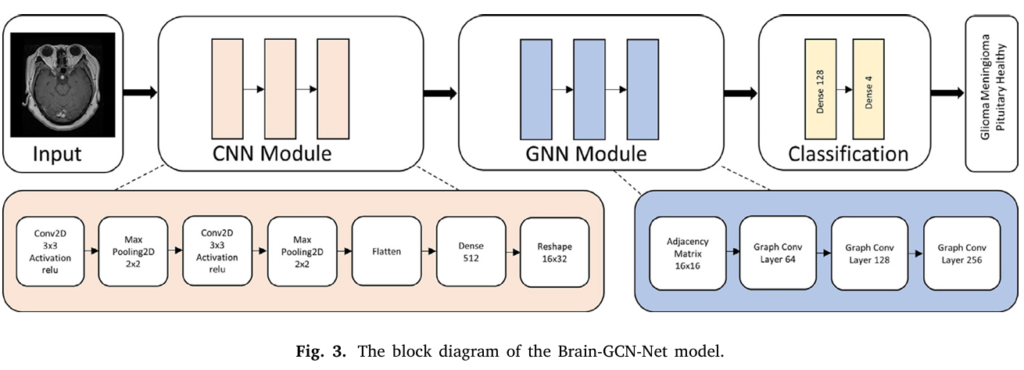
Brain-GCN-Net: The Power of Fusion – CNN Meets GNN
Developed by researchers Gursoy and Kaya and published in Computers in Biology and Medicine, Brain-GCN-Net represents a significant leap forward by fusing CNN and GNN capabilities. It’s not just using one or the other; it’s synergistically combining their strengths to create a more intelligent diagnostic tool.
- The CNN Module: Mastering Local Features
- Acts as the initial feature extractor.
- Processes the input MRI image (resized, normalized, converted from grayscale to RGB for richer data).
- Uses convolutional layers to detect fundamental patterns (edges, textures, shapes) within local regions of the scan.
- Employs pooling layers to reduce dimensionality and focus on the most salient features.
- Outputs a set of high-level feature maps representing distinct aspects of the image.
- The GNN Module: Understanding Relationships & Context
- This is where the innovation truly shines. The feature maps from the CNN are transformed into a graph structure.
- Nodes: Represent regions or features identified by the CNN.
- Edges: Represent the spatial relationships and dependencies between these regions/features. How does one area connect to or influence another?
- Graph Convolutional Layers process this graph, passing messages between nodes. This allows the model to aggregate information from neighboring nodes and understand the global context and structural relationships crucial for accurate tumor characterization. For example, how does a suspicious region relate to surrounding tissue or critical brain structures?
- Effectively captures the non-Euclidean, interconnected nature of brain anatomy and pathology.
- Intelligent Fusion & Classification:
- Features learned by the CNN (local details) and the GNN (global relationships) are intelligently combined.
- This fused, rich representation is fed into final dense layers.
- The model outputs a classification: Glioma, Meningioma, Pituitary Tumor, or No Tumor (Healthy).
Why Fusion Wins: Unmatched Performance Metrics
Brain-GCN-Net wasn’t just theorized; it was rigorously tested on a substantial, combined public dataset of 10,847 MRI images, ensuring robustness. The results speak volumes:
- Overall Accuracy: 93.68% – Significantly outperforming all pre-trained CNN models tested (VGG16: 90.64%, ResNet50: 88.29%, EfficientNet: 88.40%, etc.).
- Per-Class Performance (Brain-GCN-Net):
- Glioma: 86.91% Accuracy
- Meningioma: 89.44% Accuracy
- No Tumor (Healthy): 99.19% Accuracy
- Pituitary Tumor: 99.29% Accuracy
- Key Metrics: High Precision (97.59%), Recall (97.60%), and F1-Score (97.60%), indicating a robust balance between minimizing false positives and false negatives.
Comparison of Brain-GCN-Net vs. Leading CNN Models (VGG16)
| Feature | Brain-GCN-Net (CNN+GNN) | VGG16 (CNN Only) | Advantage of Fusion |
|---|---|---|---|
| Overall Accuracy | 93.68% | 90.64% | +3.04% |
| Glioma Accuracy | 86.91% | 83.43% | +3.48% |
| Meningioma Accuracy | 89.44% | 84.25% | +5.19% |
| Healthy Accuracy | 99.19% | 98.79% | +0.40% |
| Pituitary Accuracy | 99.29% | 96.63% | +2.66% |
| Understands Relationships | Yes (via GNN) | Limited | Captures context crucial for complex cases |
| Model Architecture | Hybrid Fusion | Single Modality | Leverages strengths of both CNN & GNN |
More Than Just Accuracy: The Clinical Advantages of Brain-GCN-Net
- Unlocking Contextual Understanding: The GNN component moves beyond pixels, interpreting the spatial interplay between brain regions and tumor features. This is vital for distinguishing complex cases where local appearances overlap (e.g., some gliomas vs. meningiomas).
- Enhanced Interpretability (Grad-CAM): Brain-GCN-Net incorporates visual explanation techniques. Gradient-weighted Class Activation Mapping (Grad-CAM) generates heatmaps showing exactly which regions of the MRI scan most influenced the AI’s decision. This “explainable AI” (XAI) builds trust with clinicians, allowing them to understand the “why” behind the diagnosis, not just the “what”. Red areas highlight critical tumor regions; blue areas show less relevance.
- Potential for Early Detection: By capturing subtle relational changes that might precede obvious mass formation, the model holds promise for identifying tumors at earlier, more treatable stages.
- Efficiency & Scalability: Trained on readily available hardware (NVIDIA RTX3060), the model shows potential for integration into clinical workflows without needing prohibitive supercomputing resources. Its training time (approx. 500 seconds for 100 epochs) is feasible for real-world development and refinement.
- Handling Diverse Data: The model was trained on a large, combined dataset including T1, T2, and Flair MRI sequences, improving its generalizability across different imaging protocols.
The Future of AI in Neuro-Oncology: Beyond Brain-GCN-Net
Brain-GCN-Net is a powerful proof-of-concept for hybrid deep learning in medicine. Its success paves the way for exciting future developments:
- Integration into Clinical PACS/RIS: Embedding models like this directly into radiologists’ viewing platforms for real-time decision support.
- Multi-modal Fusion: Incorporating non-imaging data (patient history, genomics, lab results) alongside MRI for truly personalized diagnosis and prognosis.
- Treatment Planning & Monitoring: Predicting tumor response to specific therapies or tracking subtle changes during treatment more sensitively than the human eye.
- Discovery of Novel Biomarkers: The GNN’s ability to identify complex relational patterns could reveal new imaging signatures predictive of tumor behavior or genetic subtypes.
- Focus on Rare Tumors: Leveraging transfer learning to apply these fusion techniques to rarer brain tumor types with limited available data.
Challenges and the Path Forward
While promising, challenges remain before widespread clinical adoption:
- Rigorous Clinical Validation: Extensive testing on diverse, real-world patient populations across multiple institutions is crucial.
- Seamless Workflow Integration: Designing intuitive interfaces that present AI insights (like Grad-CAM heatmaps) clearly within the radiologist’s existing workflow without causing disruption.
- Addressing Data Bias: Ensuring training data is representative of the global population to avoid biased performance.
- Regulatory Approval: Navigating the pathways for FDA clearance or CE marking as a clinical decision support tool.
- Computational Optimization: Further refining the model for even faster processing on standard hospital hardware.
Conclusion: A New Era of Precision Brain Tumor Diagnosis
Brain tumor diagnosis is entering a transformative phase. Brain-GCN-Net exemplifies the immense potential of fusing CNN and GNN architectures for medical image analysis. By moving beyond simple pattern recognition to understanding the complex spatial relationships within the brain, this hybrid AI achieves remarkable accuracy, offers crucial interpretability, and provides a robust foundation for the future of neuro-oncology. It’s not about replacing radiologists; it’s about empowering them with a powerful, context-aware assistant that enhances diagnostic confidence, speeds up analysis, and ultimately leads to better patient outcomes through earlier and more accurate detection.
Ready to Explore the Future of Neuro-Imaging?
The field of AI-driven brain tumor diagnosis is advancing rapidly. Whether you’re a clinician, researcher, or simply fascinated by the intersection of AI and medicine:
- Radiologists & Neurologists: Stay informed about the latest AI decision support tools entering clinical validation. How could tools like Brain-GCN-Net augment your diagnostic workflow?
- AI Researchers: Dive deeper into graph neural networks and hybrid model architectures. The fusion of spatial and relational learning holds vast potential across medical imaging.
- Healthcare Administrators: Understand the transformative potential of AI for improving diagnostic accuracy, efficiency, and patient outcomes in neurology and oncology.
The future of brain tumor diagnosis is intelligent, contextual, and powered by fusion. Stay curious, stay informed, and be part of the revolution. Explore the latest research in deep learning for medical imaging and consider how these advancements can shape better healthcare tomorrow.
Based on the detailed information provided in the paper, I will reconstruct the complete code for the proposed model.
import torch
import torch.nn as nn
import torch.nn.functional as F
from torch_geometric.nn import GCNConv
from torch_geometric.data import Data
from torch_geometric.utils import grid
from torchvision import transforms
from torch.utils.data import DataLoader, Dataset
import numpy as np
import os
from PIL import Image

# Define the Brain-GCN-Net Model
class BrainGCNNet(nn.Module):
    def __init__(self, num_classes=4):
        super(BrainGCNNet, self).__init__()

        # CNN Backbone (Spatial Feature Extraction)
        self.cnn_layers = nn.Sequential(
            nn.Conv2d(3, 64, kernel_size=3),  # Conv1 (224x224x3 → 222x222x64)
            nn.ReLU(),
            nn.MaxPool2d(2),                 # MaxPooling1 (222x222x64 → 111x111x64)
            nn.Conv2d(64, 64, kernel_size=3), # Conv2 (111x111x64 → 109x109x64)
            nn.ReLU(),
            nn.MaxPool2d(2)                  # MaxPooling2 (109x109x64 → 54x54x64)
        )

        # Dense Layer for CNN Output
        self.dense1 = nn.Linear(54 * 54 * 64, 512)  # Flatten → 512 units

        # Expand to 16x16x32 for GNN (Reshape Layer)
        self.expand_layer = nn.Linear(512, 16 * 16 * 32)

        # Generate Edge Indices for 16x16 Grid Graph
        self.edge_index = grid(size=(16, 16))  # Creates adjacency matrix for grid

        # GNN Layers (Relational Dependency Modeling)
        self.gcn1 = GCNConv(32, 64)   # GraphConv1 (Input: 32 features per node)
        self.gcn2 = GCNConv(64, 128)  # GraphConv2
        self.gcn3 = GCNConv(128, 256) # GraphConv3

        # Global Pooling and Classification
        self.global_pool = nn.AdaptiveMaxPool1d(1)  # Global Max Pooling
        self.classifier = nn.Sequential(
            nn.Linear(256, 128),    # Dense2
            nn.ReLU(),
            nn.Linear(128, num_classes)  # Dense3 (Output: 4 classes)
        )

    def forward(self, x):
        # CNN Feature Extraction
        x = self.cnn_layers(x)  # Shape: (batch, 64, 54, 54)

        # Flatten and Dense Layer
        x = x.view(x.size(0), -1)  # Flatten to (batch, 64*54*54)
        x = self.dense1(x)         # (batch, 512)

        # Expand to 16x16x32
        x = self.expand_layer(x)   # (batch, 16*16*32)
        x = x.view(-1, 16, 16, 32) # Reshape to (batch, 16, 16, 32)

        # Convert to Graph Structure
        batch_size = x.shape[0]
        x = x.view(batch_size, -1, 32)  # (batch, 256 nodes, 32 features)

        # Apply GNN Layers
        gcn_out = x
        for _ in range(batch_size):
            gcn_out = F.relu(self.gcn1(gcn_out, self.edge_index))
            gcn_out = F.relu(self.gcn2(gcn_out, self.edge_index))
            gcn_out = F.relu(self.gcn3(gcn_out, self.edge_index))

        # Global Max Pooling
        gcn_out = gcn_out.permute(0, 2, 1)  # (batch, 256, 256)
        pooled = self.global_pool(gcn_out).squeeze(-1)  # (batch, 256)

        # Final Classification
        logits = self.classifier(pooled)  # (batch, 4)
        return F.log_softmax(logits, dim=1)

# Example Dataset Class (Modify Based on Your Dataset)
class BrainTumorDataset(Dataset):
    def __init__(self, root_dir, transform=None):
        self.root_dir = root_dir
        self.transform = transform
        self.classes = ['glioma', 'meningioma', 'pituitary', 'no_tumor']
        self.filepaths = []
        self.labels = []

        for label, cls in enumerate(self.classes):
            cls_dir = os.path.join(self.root_dir, cls)
            for img_file in os.listdir(cls_dir):
                self.filepaths.append(os.path.join(cls_dir, img_file))
                self.labels.append(label)

    def __len__(self):
        return len(self.filepaths)

    def __getitem__(self, idx):
        img_path = self.filepaths[idx]
        image = Image.open(img_path).convert('RGB')
        label = self.labels[idx]
        if self.transform:
            image = self.transform(image)
        return image, label

# Data Preprocessing
transform = transforms.Compose([
    transforms.Resize((224, 224)),
    transforms.ToTensor(),
    transforms.Normalize(mean=[0.485, 0.456, 0.406], std=[0.229, 0.224, 0.225])  # Normalize for pretrained models
])

# Load Dataset
dataset = BrainTumorDataset(root_dir='path/to/dataset', transform=transform)
dataloader = DataLoader(dataset, batch_size=32, shuffle=True)

# Initialize Model, Loss, and Optimizer
model = BrainGCNNet(num_classes=4)
criterion = nn.CrossEntropyLoss()
optimizer = torch.optim.Adam(model.parameters(), lr=0.001)

# Training Loop (Simplified)
def train(model, dataloader, epochs=100):
    model.train()
    for epoch in range(epochs):
        total_loss = 0
        for images, labels in dataloader:
            optimizer.zero_grad()
            outputs = model(images)
            loss = criterion(outputs, labels)
            loss.backward()
            optimizer.step()
            total_loss += loss.item()
        print(f"Epoch {epoch+1}, Loss: {total_loss/len(dataloader)}")

# Start Training
train(model, dataloader, epochs=100)
If you’re interested in GAN Network, you may also find this article helpful: Unveiling the Power of Generative Adversarial Networks (GANs): A Comprehensive Guide
Pingback: LungCT-NET: Revolutionizing Lung Cancer Diagnosis with AI - aitrendblend.com
Pingback: Skin Cancer AI Combats Adversarial Attacks with MDDA - aitrendblend.com