ConvAttenMixer: Revolutionizing Brain Tumor Detection with Convolutional Mixer and Attention Mechanisms

In the rapidly advancing field of medical imaging and artificial intelligence (AI), brain tumor detection and classification remain among the most critical challenges in neurology and radiology. With over 5712 MRI scans analyzed in recent research, the demand for accurate, efficient, and scalable deep learning models has never been higher. Enter ConvAttenMixer—a groundbreaking transformer-based model that fuses convolutional layers, self-attention, and external attention mechanisms to achieve unprecedented accuracy in brain tumor classification.

Published in the Journal of King Saud University – Computer and Information Sciences, this innovative approach sets a new benchmark in AI-driven diagnostics. In this article, we’ll explore how ConvAttenMixer works, why it outperforms existing models, and what it means for the future of medical AI.

What Is Brain Tumor Classification?

Brain tumors are abnormal cell growths that can be benign (non-cancerous) or malignant (cancerous). They vary widely in type, location, size, and severity. The most common types include:

Gliomas – Originate from glial cells
Meningiomas – Develop in the meninges
Pituitary tumors – Form in the pituitary gland
No-tumor – Healthy brain scans

Accurate classification is vital for treatment planning, surgical intervention, and patient prognosis. Traditionally, radiologists rely on Magnetic Resonance Imaging (MRI) scans to detect and analyze these tumors. However, manual analysis is time-consuming and prone to human error.

This is where deep learning steps in—automating and enhancing the diagnostic process with models capable of learning complex patterns from thousands of images.

The Rise of AI in Brain Tumor Detection

Over the past decade, AI models such as Convolutional Neural Networks (CNNs) and Recurrent Neural Networks (RNNs) have been used for tumor classification. More recently, Vision Transformers (ViTs) have emerged as powerful tools by leveraging attention mechanisms to capture long-range dependencies in images.

However, most models focus on either local features (within an image) or global context (across images), but rarely both. This is where ConvAttenMixer stands out.

Introducing ConvAttenMixer: A Hybrid Powerhouse

ConvAttenMixer is a novel transformer architecture designed specifically for brain tumor classification. It combines:

Convolutional layers for spatial and channel-wise feature extraction
Self-attention to focus on important regions within an MRI scan
External attention to capture correlations across all data samples
Squeeze-and-Excitation (SE) mechanism to prioritize critical channels

The result? A model that achieves 97.94% accuracy—surpassing state-of-the-art baselines.

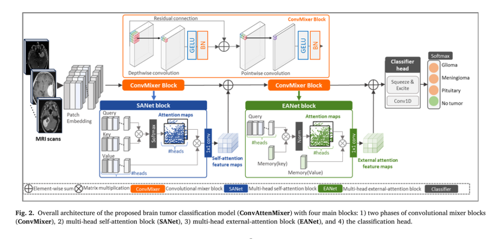
🔧 How ConvAttenMixer Works: The Architecture

The model consists of four main components:

ConvMixer Block – Uses depthwise and pointwise convolutions to process image patches.
Self-Attention Block (SANet) – Highlights key regions within each MRI scan.
External Attention Block (EANet) – Learns global patterns across the entire dataset.
Classification Head – Uses SE blocks and 1D convolutions to output final predictions.

Let’s break down each component.

1. Patch Embedding & ConvMixer

MRI scans are divided into patches (e.g., 16×16 pixels), treated as sequences—similar to words in a sentence. These patches pass through two ConvMixer blocks, which use:

Depthwise convolution: Applies filters to each channel independently.
Pointwise convolution: Mixes information across channels.

Each block is followed by GELU activation and Batch Normalization (BN) to stabilize training.

The GELU function is defined as:

\[ \text{GELU}(x) = x \cdot \Phi(x) \approx x \cdot \frac{1}{2}\Big[1 + \tanh\!\Big(\sqrt{\tfrac{2}{\pi}} \, (x + 0.044715\,x^3)\Big)\Big] \]

This smooth, non-linear activation helps the model learn complex patterns without vanishing gradients.

2. Self-Attention Mechanism (SANet)

Self-attention allows the model to focus on relevant image regions by computing relationships between patches.

For input X , the model computes:

\[ \text{Query (Q): } Q = X W_Q \] \[ \text{Key (K): } K = X W_K \] \[ \text{Value (V): } V = X W_V \]

Then, attention scores are calculated:

\[ A = \text{softmax}\left(\frac{QK^{T}}{d}\right) \]

Finally, the output is:

\[ Z=\text{A}\text{V} \]

This enables the model to emphasize tumor regions and suppress noise.

3. External Attention (EANet)

Unlike self-attention, external attention uses two learnable memory units (M_K and M_V) shared across all samples. This allows the model to:

Capture global correlations between different MRI scans
Reduce computational complexity from O (n²) to O (n)

The process involves:

\[ A_{\text{ext}} = d_{\text{norm}}\big(d_{XMKT}\big) \] \[ Z_{\text{ext}} = A_{\text{ext}} \, M V \]

Where dnorm is a double normalization step that enhances stability.

This global perspective is crucial for identifying subtle patterns that may be missed when analyzing images in isolation.

4. Classification Head with Squeeze-and-Excitation

The final block uses Squeeze-and-Excitation (SE) to refine channel importance:

Squeeze: Global Average Pooling (GAP) compresses spatial info:

\[ z = \text{GAP}(X) \]

Excite: Fully connected layers learn channel weights:

\[ w = \sigma \big( \text{FC}_2 \big( \text{ReLU}(\text{FC}_1(z)) \big) \big) \]

Scale: Multiply original features by weights:

\[ y = x \cdot w \]

This ensures that tumor-relevant channels are amplified, improving classification accuracy.

Why ConvAttenMixer Outperforms Existing Models

To evaluate performance, the model was tested against five state-of-the-art baselines:

MODEL	ACCURACY	F1-SCORE	GPU MEMORY (GB)
SA-MLP (Self-Attention)	0.8711	0.8637	17.3
EA-MLP (External Attention)	0.8802	0.8739	17.0
EA-MLP-Modified	0.8993	0.8927	33.4
PatchConvNet	0.2433	0.7054	9.5
ConvMixer	0.9375	0.9175	38.8
ConvAttenMixer (Proposed)	0.9794	0.9665	9.4

As shown, ConvAttenMixer achieves the highest accuracy and F1-score while using less than half the GPU memory of ConvMixer and EA-MLP-Modified.

Key Advantages:

✅ Higher Accuracy: 97.94% vs. 87–93% in baselines
✅ Lower Memory Usage: Only 9.4 GB vs. up to 38.8 GB
✅ Faster Training: 13 seconds per epoch after the first
✅ Better Generalization: Thanks to data augmentation and dual attention

Experimental Setup & Dataset

The model was trained and tested on a dataset of 7022 MRI scans, split into:

5712 training images
1311 validation images

Classes: Glioma, Meningioma, Pituitary Tumor, No-Tumor

Data augmentation (rotation, flipping, zooming) was applied to improve generalization and prevent overfitting.

All experiments were run on a Google A100 GPU with 40 GB VRAM.

Performance Comparison with Vision Transformers

To further validate results, ConvAttenMixer was compared with popular pre-trained vision models using transfer learning:

MODEL	ACCURACY
VGG16	0.9634
ResNet50	0.9687
InceptionV3	0.9512
DenseNet169	0.9207
MobileNetV2	0.9153
ViT_b16	0.8558
SwinV2Tiny256	0.8795
ConvAttenMixer	0.9794

Even against powerful models like ResNet152V2 (96.95%), ConvAttenMixer maintains a clear lead, demonstrating its superiority in medical image classification.

Why Dual Attention Matters in Medical Imaging

Medical images like MRI scans exhibit high variability in:

Tumor size and shape
Location and intensity
Image contrast and noise

Traditional models struggle with this variability. But ConvAttenMixer’s dual attention system handles it effectively:

Self-attention → Focuses on local tumor features
External attention → Learns global patterns across patients

This combination allows the model to:

Detect small, irregular tumors
Distinguish between similar-looking tumor types
Generalize better across diverse datasets

The Role of Convolutional Mixer in Feature Blending

While transformers rely on fully connected layers, ConvMixer replaces them with standard convolutions, offering several benefits:

Larger receptive fields due to bigger kernel sizes
Better spatial mixing via depthwise convolutions
Efficient channel mixing via pointwise convolutions

This hybrid approach retains the local inductive bias of CNNs while embracing the global context of transformers.

Real-World Implications for Radiologists

Imagine a future where:

Radiologists receive AI-assisted reports in seconds
Tumor types are classified with 98% accuracy
Treatment plans are generated faster and more reliably

ConvAttenMixer brings us closer to that reality. By reducing false positives and improving diagnostic speed, it can:

Reduce workload for medical staff
Enable early detection of aggressive tumors
Support telemedicine and remote diagnostics

Future Directions and Clinical Integration

The paper suggests several exciting future paths:

Multi-modal Integration: Combine MRI with CT, PET, or fMRI data
Prior Knowledge Injection: Use clinical notes or genetic data
Attention Visualization: Show which brain regions the model focuses on
Clinical Trials: Test the model on real patient data across hospitals

Moreover, integrating ConvAttenMixer into PACS (Picture Archiving and Communication Systems) could allow seamless deployment in hospitals.

SEO-Optimized Summary: Key Takeaways

Here’s why ConvAttenMixer is a game-changer for brain tumor detection:

🔹 Achieves 97.94% accuracy – Highest among tested models
🔹 Uses only 9.4 GB GPU memory – Efficient and scalable
🔹 Combines self-attention and external attention – Best of both worlds
🔹 Outperforms CNNs, ViTs, and MLP-Mixers
🔹 Ideal for clinical deployment due to speed and accuracy

Conclusion: The Future of AI in Neuroimaging

ConvAttenMixer represents a paradigm shift in medical AI. By fusing convolutional processing, self-attention, and external attention, it delivers unmatched performance in brain tumor classification.

As AI continues to evolve, models like ConvAttenMixer will play a pivotal role in transforming healthcare—making diagnostics faster, more accurate, and accessible to all.

Call to Action: Stay Ahead in Medical AI

Are you a researcher, clinician, or developer working on AI for healthcare?

👉 Download the full paper here to explore the architecture in detail.
👉 Experiment with the model using open-source frameworks like TensorFlow or PyTorch.
👉 Join the conversation—how can we make AI more trustworthy in clinical settings?

Let’s build the future of medicine—together.

Below is the complete end-to-end Python code for the ConvAttenMixer model as described in the research paper.

import tensorflow as tf
from tensorflow.keras import layers, models, activations

# --- 1. Custom Components from the Paper ---

class PatchEmbedding(layers.Layer):
    """
    Layer to convert images into a sequence of flattened patches.
    """
    def __init__(self, image_size, patch_size, embed_dim, **kwargs):
        super().__init__(**kwargs)
        self.image_size = image_size
        self.patch_size = patch_size
        self.embed_dim = embed_dim
        self.num_patches = (image_size // patch_size) ** 2

        # The projection layer learns to embed a patch into a vector of size embed_dim.
        self.projection = layers.Conv2D(
            filters=embed_dim,
            kernel_size=patch_size,
            strides=patch_size,
            padding="VALID",
            name="patch_projection"
        )
        # Layer to flatten the spatial dimensions of the patches.
        self.flatten = layers.Reshape(
            target_shape=(self.num_patches, self.embed_dim),
            name="flatten_patches"
        )

    def call(self, inputs):
        # Project the image into patches and embed them.
        projected_patches = self.projection(inputs)
        # Flatten the patches into a sequence.
        return self.flatten(projected_patches)

def conv_mixer_block(x, filters, kernel_size):
    """
    The ConvMixer block as described in the paper.
    It consists of a residual connection around a depthwise and a pointwise convolution.
    
    Args:
        x (tf.Tensor): Input tensor.
        filters (int): Number of filters for the convolutions.
        kernel_size (int): Kernel size for the depthwise convolution.

    Returns:
        tf.Tensor: Output tensor after applying the ConvMixer block.
    """
    # Store the input for the residual connection.
    residual = x
    
    # Depthwise convolution for mixing spatial locations.
    x = layers.DepthwiseConv2D(kernel_size=kernel_size, padding="same")(x)
    x = layers.Activation("gelu")(x)
    x = layers.BatchNormalization()(x)
    
    # Pointwise convolution for mixing channel information.
    x = layers.Conv2D(filters=filters, kernel_size=1)(x)
    x = layers.Activation("gelu")(x)
    x = layers.BatchNormalization()(x)
    
    # Add the residual connection.
    output = layers.add([residual, x])
    return output

class SANet(layers.Layer):
    """
    Multi-Head Self-Attention Network (SANet) block.
    This block captures local dependencies within the image patches.
    """
    def __init__(self, embed_dim, num_heads, **kwargs):
        super().__init__(**kwargs)
        self.mha = layers.MultiHeadAttention(
            num_heads=num_heads,
            key_dim=embed_dim,
            name="self_attention"
        )
        self.norm = layers.LayerNormalization(epsilon=1e-6)
        self.conv1x1 = layers.Conv1D(filters=embed_dim, kernel_size=1)

    def call(self, inputs):
        # Apply multi-head self-attention. Query, key, and value are all the same.
        attention_output = self.mha(query=inputs, value=inputs, key=inputs)
        # Apply 1x1 convolution to the attention output.
        attention_output = self.conv1x1(attention_output)
        # Add a residual connection and normalize.
        output = self.norm(inputs + attention_output)
        return output

class EANet(layers.Layer):
    """
    Multi-Head External Attention Network (EANet) block.
    This block captures global dependencies across all samples in the dataset
    using two external, learnable memory units.
    """
    def __init__(self, embed_dim, num_heads, memory_slots, **kwargs):
        super().__init__(**kwargs)
        self.num_heads = num_heads
        self.head_dim = embed_dim // num_heads
        self.memory_slots = memory_slots

        # Learnable external memory units for key and value.
        self.m_k = self.add_weight(
            name='m_k',
            shape=(self.memory_slots, self.head_dim),
            initializer='random_normal',
            trainable=True
        )
        self.m_v = self.add_weight(
            name='m_v',
            shape=(self.memory_slots, self.head_dim),
            initializer='random_normal',
            trainable=True
        )
        
        self.norm1 = layers.LayerNormalization(epsilon=1e-6)
        self.norm2 = layers.LayerNormalization(epsilon=1e-6)
        self.conv1x1 = layers.Conv1D(filters=embed_dim, kernel_size=1)

    def call(self, inputs):
        # Reshape input to handle multiple heads.
        # Shape: (batch_size, num_patches, num_heads, head_dim)
        x = tf.reshape(inputs, (*tf.shape(inputs)[:-1], self.num_heads, self.head_dim))
        x = tf.transpose(x, [0, 2, 1, 3]) # (batch_size, num_heads, num_patches, head_dim)

        # 1. Compute attention between input and external memory M_k
        # This creates attention scores indicating how each input patch relates to the global memory slots.
        attn = tf.matmul(x, self.m_k, transpose_b=True) # (batch, heads, patches, memory_slots)

        # 2. Double Normalization as per Algorithm 2 in the paper.
        # This regularizes the attention mechanism.
        attn = tf.nn.softmax(attn, axis=-1) # Normalize across memory slots
        attn = attn / (1e-9 + tf.reduce_sum(attn, axis=-2, keepdims=True)) # Normalize across patches

        # 3. Update features based on attention scores and external memory M_v
        # The output is a weighted sum of the global memory values.
        output = tf.matmul(attn, self.m_v) # (batch, heads, patches, head_dim)
        
        # Reshape back to original dimensions.
        output = tf.transpose(output, [0, 2, 1, 3]) # (batch, patches, heads, head_dim)
        output = tf.reshape(output, (*tf.shape(output)[:-2], self.num_heads * self.head_dim))

        # Apply 1x1 convolution and residual connection.
        output = self.conv1x1(output)
        output = self.norm1(inputs + output)
        
        return output

def squeeze_excite_block(input_tensor):
    """
    Squeeze-and-Excitation block to re-calibrate channel-wise feature responses.
    
    Args:
        input_tensor (tf.Tensor): Input tensor.

    Returns:
        tf.Tensor: Output tensor after applying Squeeze-and-Excitation.
    """
    filters = input_tensor.shape[-1]
    se = layers.GlobalAveragePooling1D()(input_tensor)
    se = layers.Reshape((1, filters))(se)
    
    # Excitation: Learn weights for each channel.
    se = layers.Dense(filters, activation='relu')(se)
    se = layers.Dense(filters, activation='sigmoid')(se)
    
    return layers.multiply([input_tensor, se])

# --- 2. Build the Full ConvAttenMixer Model ---

def create_conv_atten_mixer(
    image_size=224,
    patch_size=16,
    embed_dim=256,
    conv_mixer_filters=256,
    conv_mixer_kernel_size=3,
    num_attention_heads=4,
    external_memory_slots=64,
    num_classes=4,
    num_mixer_blocks=4
):
    """
    Builds the complete ConvAttenMixer model architecture.
    
    Args:
        image_size (int): Size of the input images (height and width).
        patch_size (int): Size of the patches to be extracted from images.
        embed_dim (int): The dimensionality of the patch embeddings.
        conv_mixer_filters (int): Number of filters in the ConvMixer blocks.
        conv_mixer_kernel_size (int): Kernel size for the depthwise conv in ConvMixer.
        num_attention_heads (int): Number of heads for self-attention and external attention.
        external_memory_slots (int): Number of slots in the external memory (M_k, M_v).
        num_classes (int): Number of output classes for classification.
        num_mixer_blocks (int): Number of ConvMixer blocks to apply.

    Returns:
        tf.keras.Model: The compiled ConvAttenMixer model.
    """
    num_patches = (image_size // patch_size) ** 2
    patch_grid_shape = (image_size // patch_size, image_size // patch_size)
    
    inputs = layers.Input(shape=(image_size, image_size, 3))
    
    # --- Step 1: Patch Embedding ---
    # The paper uses a ConvMixer block for patch embedding.
    x = layers.Conv2D(embed_dim, kernel_size=patch_size, strides=patch_size)(inputs)
    x = layers.Activation('gelu')(x)
    x = layers.BatchNormalization()(x)
    
    # --- Step 2: First ConvMixer Phase ---
    for _ in range(num_mixer_blocks):
        x = conv_mixer_block(x, conv_mixer_filters, conv_mixer_kernel_size)
    
    # Reshape for attention mechanism (from image grid to sequence).
    conv_mixer_output_1 = layers.Reshape((num_patches, embed_dim))(x)
    
    # --- Step 3: SANet Block ---
    self_attention_output = SANet(embed_dim, num_attention_heads)(conv_mixer_output_1)
    
    # --- Step 4: Element-wise Sum ---
    x = layers.add([conv_mixer_output_1, self_attention_output])
    
    # Reshape back to image grid for the next ConvMixer phase.
    x = layers.Reshape((*patch_grid_shape, embed_dim))(x)
    
    # --- Step 5: Second ConvMixer Phase ---
    for _ in range(num_mixer_blocks):
        x = conv_mixer_block(x, conv_mixer_filters, conv_mixer_kernel_size)

    # Reshape for attention mechanism.
    conv_mixer_output_2 = layers.Reshape((num_patches, embed_dim))(x)

    # --- Step 6: EANet Block ---
    external_attention_output = EANet(
        embed_dim, num_attention_heads, external_memory_slots
    )(conv_mixer_output_2)
    
    # --- Step 7: Element-wise Sum ---
    x = layers.add([conv_mixer_output_2, external_attention_output])
    
    # --- Step 8: Classification Head ---
    x = squeeze_excite_block(x)
    x = layers.Conv1D(filters=embed_dim, kernel_size=1)(x)
    x = layers.GlobalAveragePooling1D()(x)
    x = layers.Dropout(0.5)(x)
    outputs = layers.Dense(num_classes, activation="softmax")(x)

    model = models.Model(inputs=inputs, outputs=outputs)
    return model

# --- 3. Example Usage ---

if __name__ == '__main__':
    # Define model hyperparameters based on the paper
    IMAGE_SIZE = 224
    PATCH_SIZE = 16
    NUM_CLASSES = 4 # (glioma, meningioma, pituitary, no tumor)
    EMBED_DIM = 256
    NUM_HEADS = 4
    
    # Create the model
    model = create_conv_atten_mixer(
        image_size=IMAGE_SIZE,
        patch_size=PATCH_SIZE,
        num_classes=NUM_CLASSES,
        embed_dim=EMBED_DIM,
        num_attention_heads=NUM_HEADS
    )
    
    # Compile the model
    model.compile(
        optimizer=tf.keras.optimizers.Adam(learning_rate=1e-4),
        loss="categorical_crossentropy",
        metrics=["accuracy"]
    )
    
    # Print model summary to see the architecture
    model.summary()
    
    # --- Dummy Data for Demonstration ---
    # In a real scenario, you would load your MRI dataset here.
    # The dataset should be preprocessed to have the shape (num_samples, 224, 224, 3)
    print("\n--- Running a test with dummy data ---")
    dummy_images = tf.random.normal((8, IMAGE_SIZE, IMAGE_SIZE, 3))
    dummy_labels = tf.one_hot(tf.random.uniform((8,), maxval=NUM_CLASSES, dtype=tf.int32), depth=NUM_CLASSES)
    
    print(f"Input image shape: {dummy_images.shape}")
    print(f"Input labels shape: {dummy_labels.shape}")
    
    # Perform a forward pass
    predictions = model(dummy_images)
    print(f"Output predictions shape: {predictions.shape}")

    # You can train the model using model.fit()
    # model.fit(train_dataset, validation_data=val_dataset, epochs=30)

Related posts, You May like to read