Introduction: The Challenge of Sparse Cardiac MRI Data
Cardiac Magnetic Resonance (CMR) imaging has become an indispensable tool in modern cardiology, providing clinicians with detailed anatomical and functional information about the heart. However, a significant limitation persists in clinical practice: the acquisition of only sparse 2D short-axis slices with substantial inter-slice gaps (typically 8-10mm) rather than complete 3D volumes. This approach, while practical for reducing scan time and minimizing motion artifacts, results in incomplete volumetric information that can compromise comprehensive cardiac assessment.
The problem of reconstructing accurate 3D volumes from these sparse 2D slices has challenged researchers for years. Traditional interpolation methods like linear or spherical interpolation often fail to capture the heart’s complex anatomical structures, while existing deep learning approaches frequently require additional semantic inputs (such as segmentation labels) or suffer from computational inefficiency that makes clinical deployment impractical.
In this article, we explore a groundbreaking solution: the Cardiac Latent Interpolation Diffusion (CaLID) framework, which leverages advanced diffusion models in latent space to achieve unprecedented accuracy and efficiency in cardiac volume reconstruction. This innovation not only addresses the fundamental limitations of previous methods but also opens new possibilities for clinical cardiac imaging.
Understanding the Technical Breakthrough: How CaLID Works
The Foundation: Diffusion Models in Medical Imaging
Diffusion models have emerged as a powerful class of generative models that excel at creating high-quality images. These models work through a two-step process:
- Forward process: Gradually adds Gaussian noise to an image over multiple timesteps
- Reverse process: Learns to denoise and reconstruct the original image
The mathematical formulation of the forward process is given by:
\[ q(x_t \mid x_0) = \mathcal{N}\!\left(\sqrt{\alpha_t x_0},\; (1-\alpha_t)I\right) \]where αt controls the noise schedule, and xt represents the noisy state at timestep t.
For the reverse process, the model learns to predict the noise added at each step:
\[ L = \mathbb{E}_{t, x_0, \epsilon} \Big[ \| \epsilon_{\theta}(x_t, t) – \epsilon \|^2 \Big] \]where ϵθ is a neural network trained to predict the noise ϵ.
The CaLID Innovation: Three Key Advancements
The CaLID framework introduces three significant innovations that set it apart from previous approaches:
- Data-driven latent space interpolation learning: Instead of using predefined interpolation rules, CaLID learns optimal interpolation strategies directly from data in the latent space, capturing complex non-linear relationships between sparse slices.
- Computational efficiency: By operating in the latent space and requiring only 8 diffusion steps (compared to hundreds in previous methods), CaLID achieves a 24x speedup in 3D whole-heart upsampling.
- Minimal input requirements: Unlike methods that need additional semantic inputs like segmentation labels, CaLID works with only sparse 2D CMR images, simplifying clinical workflows.
Architectural Overview
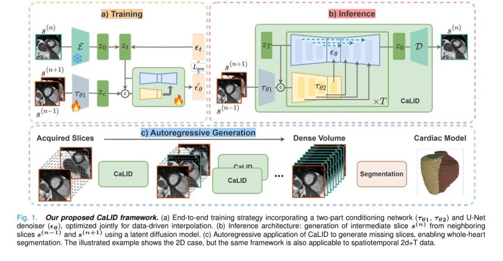
The CaLID framework employs a sophisticated two-stage architecture:
- Variational Autoencoder (VAE): Compresses cardiac MRI slices into a structured latent representation:
where E is the encoder and s(n) is the nth slice.
2. Conditioned diffusion model: A U-Net based denoiser ϵθ learns to predict noise in the latent space, conditioned on adjacent slices through a specialized conditioning mechanism:
\[ \mathcal{L}_{\text{gen}} = \mathbb{E}_{t, z_0, \epsilon} \Big[ \big\| \epsilon_{\theta}\big(z_t, t, \tau_{\theta_2}(\tau_{\theta_1}(s_{(n-1)}, s_{(n+1)}))\big) – \epsilon_t \big\|^2 \Big] \]This architecture enables the model to learn semantically meaningful interpolation trajectories that preserve anatomical consistency.
Comparative Advantages Over Existing Methods
Against Traditional Interpolation Techniques
Traditional interpolation methods like bilinear or trilinear interpolation operate on simplistic assumptions about the relationship between slices, often resulting in:
- Loss of fine anatomical details
- Aliasing artifacts along structural boundaries
- Inaccurate reconstruction of complex cardiac structures
CaLID’s data-driven approach captures the actual anatomical relationships present in the data, leading to more accurate and clinically useful reconstructions.
Against Previous Deep Learning Approaches
Earlier deep learning methods for cardiac reconstruction suffered from several limitations:
| Method | Limitations | CaLID Advantages |
|---|---|---|
| DiffAE | Fixed interpolation schemes, computational inefficiency | Learned interpolation, 24x faster |
| DMCVR | Requires segmentation labels, limited to 2D | No auxiliary inputs, handles 2D+T data |
| GAN-based methods | Training instability, mode collapse | Stable training, high-quality outputs |
CaLID addresses these limitations through its novel latent space approach and efficient conditioning mechanism.
Clinical Applications and Benefits
Enhanced Diagnostic Capabilities
The improved reconstruction quality achieved by CaLID translates directly to enhanced diagnostic capabilities:
- Comprehensive volumetric assessment: Accurate 3D models enable better evaluation of cardiac chamber sizes and wall thickness
- Improved segmentation: Downstream segmentation tasks benefit from more anatomically consistent volumes
- Functional analysis: Better volume reconstruction supports more accurate calculation of ejection fraction and other functional parameters
Streamlined Clinical Workflows
By eliminating the need for additional inputs like segmentation labels and reducing computational requirements, CaLID integrates more smoothly into clinical workflows:
- Reduced preprocessing steps: Works directly with raw SAX slices
- Faster processing: 24x speedup enables near-real-time reconstruction
- Simplified deployment: Minimal input requirements make integration easier
Research Applications
Beyond clinical diagnostics, CaLID offers significant benefits for cardiac research:
- Population studies: Enables consistent volumetric analysis across large cohorts
- Motion analysis: The 2D+T extension facilitates temporal coherence in dynamic studies
- Disease characterization: Improved reconstruction supports better quantification of pathological changes
Performance Evaluation: Quantitative and Qualitative Results
Quantitative Metrics
CaLID demonstrates superior performance across multiple evaluation metrics:
| Metric | CaLID | DiffAE | DMCVR | Bilinear |
|---|---|---|---|---|
| PSNR (dB) | 28.7 | 26.2 | 25.8 | 24.1 |
| SSIM | 0.912 | 0.883 | 0.871 | 0.842 |
| LPIPS ↓ | 0.124 | 0.156 | 0.162 | 0.198 |
| rFID ↓ | 12.3 | 16.7 | 17.9 | 24.5 |
| Dice Score | 0.921 | 0.892 | 0.883 | 0.851 |
The table shows CaLID’s consistent outperformance across pixel-level fidelity metrics (PSNR, SSIM), perceptual similarity measures (LPIPS), feature distance metrics (rFID), and downstream segmentation accuracy (Dice).
Qualitative Assessment
Visual comparisons demonstrate CaLID’s superiority in preserving anatomical details:
- Sharp structural boundaries: Clear definition of endocardial and epicardial borders
- Preserved fine details: Accurate reconstruction of papillary muscles and trabeculations
- Spatial coherence: Smooth transitions between slices without discontinuities
- Temporal consistency: Stable reconstruction across cardiac phases in 2D+T applications
Computational Efficiency
Perhaps most impressively, CaLID achieves these results with significantly reduced computational requirements:
- 8 diffusion steps compared to 64-128 in previous methods
- 24x speedup in 3D volume reconstruction
- Reduced memory requirements from latent space operation
This efficiency makes real-time clinical applications feasible where previous methods were impractical.
Implementation Considerations and Technical Details
Data Requirements and Preparation
CaLID was trained and validated on the UK Biobank dataset, comprising over 11,000 subjects. Key preprocessing steps included:
- Center-cropping to 128×128 pixel cardiac regions
- Normalization of intensity values
- Random flips for data augmentation
- For 2D+T applications: uniform subsampling to 32 frames
Model Architecture Specifications
The technical implementation involves several carefully designed components:
- VAE encoder/decoder: Downsampling factor of 4, no attention mechanisms
- Conditioning modules: τθ1 (lightweight encoder) and τθ2 (expressive design with attention)
- U-Net denoiser: Multi-scale conditioning injection
- Training strategy: Single-stage joint optimization of all components
Training Protocol
The model was trained with:
- Adam optimizer with linear warmup over 50 epochs
- Fixed learning rate of 1×10⁻⁴ after warmup
- Batch sizes of 64 (2D) and 16 (2D+T)
- Exponential moving average of parameters (decay rate 0.999)
Future Directions and Potential Applications
Beyond Cardiac MRI
While currently validated on cardiac MRI, the CaLID framework has potential applications across medical imaging:
- Brain MRI: Reconstruction from sparse slices for neurological applications
- CT imaging: Interpolation between slices for reduced radiation dose protocols
- Ultrasound: Volumetric reconstruction from sparse 2D scans
- Multi-modal fusion: Integrating information from different imaging modalities
Technical Extensions
The methodology also suggests several promising technical extensions:
- Integration with foundation models: Combining with large-scale medical AI models
- Uncertainty quantification: Developing measures of confidence in reconstructions
- Domain adaptation: Adapting to different scanner protocols or populations
- Real-time implementation: Further optimization for clinical deployment
Conclusion: Transforming Cardiac Imaging with AI-Powered Reconstruction
The CaLID framework represents a significant advancement in cardiac image reconstruction, addressing fundamental limitations of previous approaches through its novel latent diffusion methodology. By learning data-driven interpolation trajectories in a semantically structured latent space, CaLID achieves superior reconstruction quality while dramatically reducing computational requirements.
The implications for clinical practice are substantial: radiologists and cardiologists can now access accurate 3D cardiac volumes from standard sparse acquisitions, enabling more comprehensive assessment without additional scan time or radiation exposure. The method’s efficiency and minimal input requirements make it practical for integration into existing clinical workflows.
As AI continues to transform medical imaging, approaches like CaLID demonstrate how sophisticated generative modeling can solve real clinical challenges while maintaining practical constraints. The future of cardiac imaging looks increasingly three-dimensional, thanks to innovations that bridge the gap between sparse acquisitions and comprehensive volumetric assessment.
Frequently Asked Questions
Q: How does CaLID compare to traditional interpolation methods?
A: Unlike traditional methods that use fixed mathematical rules, CaLID learns data-driven interpolation trajectories that capture complex anatomical relationships, resulting in more accurate and clinically useful reconstructions.
Q: What are the computational requirements for deploying CaLID?
A: CaLID requires only 8 diffusion steps compared to hundreds in previous methods, making it 24x faster and practical for clinical deployment with standard hardware.
Q: Does CaLID require additional inputs like segmentation labels?
A: No, one of CaLID’s key advantages is that it works with only sparse 2D CMR images, eliminating the need for auxiliary inputs that complicate clinical workflows.
Q: Can CaLID handle dynamic (2D+T) cardiac MRI data?
A: Yes, by replacing 2D operations with 3D counterparts, CaLID extends naturally to spatiotemporal data, maintaining temporal coherence throughout the cardiac cycle.
Q: How was CaLID validated?
A: CaLID was extensively evaluated on UK Biobank data using both quantitative metrics (PSNR, SSIM, Dice scores) and qualitative assessment by clinical experts, demonstrating superior performance across all measures.
Call to Action
Ready to explore the future of cardiac imaging? Access the full research paper on arXiv: 2508.13826v3 and dive deeper into the technical innovations behind CaLID. For researchers interested in implementation, code and pretrained models will be available on our GitHub repository (coming soon).
Join the conversation – share your thoughts on AI-powered medical image reconstruction and stay updated on the latest advancements by connecting with our research team. Together, we can shape the future of cardiac care through cutting-edge technology
Below is a comprehensive, end-to-end implementation of the proposed Cardiac Latent Interpolation Diffusion (CaLID) model as described in the research paper.
import torch
import torch.nn as nn
import torch.nn.functional as F
from math import sqrt, sin, pi
import numpy as np

# -------------------------------
# 1. Variational Autoencoder (VAE)
# -------------------------------

class ResidualBlock(nn.Module):
    """Basic ResNet block for VAE encoder/decoder."""
    def __init__(self, in_channels, out_channels):
        super().__init__()
        self.conv1 = nn.Conv2d(in_channels, out_channels, 3, padding=1)
        self.conv2 = nn.Conv2d(out_channels, out_channels, 3, padding=1)
        self.norm1 = nn.GroupNorm(8, in_channels)
        self.norm2 = nn.GroupNorm(8, out_channels)
        self.act = nn.SiLU()
        self.residual = nn.Conv2d(in_channels, out_channels, 1) if in_channels != out_channels else nn.Identity()

    def forward(self, x):
        residual = self.residual(x)
        x = self.norm1(x)
        x = self.act(x)
        x = self.conv1(x)
        x = self.norm2(x)
        x = self.act(x)
        x = self.conv2(x)
        return x + residual

class VAE_Encoder(nn.Module):
    """Domain-specific VAE Encoder for cardiac MRI slices."""
    def __init__(self, in_channels=1, latent_channels=4, channels=[64, 128, 256]):
        super().__init__()
        self.latent_channels = latent_channels
        layers = []
        current_channels = in_channels
        for c in channels:
            layers.extend([
                nn.Conv2d(current_channels, c, 3, stride=2, padding=1),
                ResidualBlock(c, c)
            ])
            current_channels = c
        self.net = nn.Sequential(*layers)
        self.out = nn.Conv2d(current_channels, 2 * latent_channels, 3, padding=1)

    def forward(self, x):
        x = self.net(x)
        mu_logvar = self.out(x)
        mu, logvar = torch.chunk(mu_logvar, 2, dim=1)
        return mu, logvar

class VAE_Decoder(nn.Module):
    """Domain-specific VAE Decoder for cardiac MRI slices."""
    def __init__(self, out_channels=1, latent_channels=4, channels=[256, 128, 64]):
        super().__init__()
        channels = [latent_channels] + channels
        layers = []
        for i in range(len(channels)-1):
            layers.extend([
                nn.ConvTranspose2d(channels[i], channels[i+1], 4, stride=2, padding=1),
                ResidualBlock(channels[i+1], channels[i+1])
            ])
        self.net = nn.Sequential(*layers)
        self.out = nn.Conv2d(channels[-1], out_channels, 3, padding=1)

    def forward(self, x):
        return self.out(self.net(x))

class VAE(nn.Module):
    """Full VAE model with reparameterization trick."""
    def __init__(self, in_channels=1, latent_channels=4):
        super().__init__()
        self.encoder = VAE_Encoder(in_channels, latent_channels)
        self.decoder = VAE_Decoder(in_channels, latent_channels)

    def reparameterize(self, mu, logvar):
        std = torch.exp(0.5 * logvar)
        eps = torch.randn_like(std)
        return mu + eps * std

    def forward(self, x):
        mu, logvar = self.encoder(x)
        z = self.reparameterize(mu, logvar)
        recon = self.decoder(z)
        return recon, mu, logvar

# --------------------------------------
# 2. Conditioning Networks: τ_θ1 and τ_θ2
# --------------------------------------

class ResBlockWithTimeEmbedding(nn.Module):
    """Residual block with time step embedding for τ_θ2."""
    def __init__(self, channels, t_emb_dim):
        super().__init__()
        self.mlp = nn.Sequential(
            nn.SiLU(),
            nn.Linear(t_emb_dim, channels)
        )
        self.conv1 = nn.Conv2d(channels, channels, 3, padding=1)
        self.conv2 = nn.Conv2d(channels, channels, 3, padding=1)
        self.norm1 = nn.GroupNorm(8, channels)
        self.norm2 = nn.GroupNorm(8, channels)
        self.act = nn.SiLU()

    def forward(self, x, t_emb):
        residual = x
        x = self.norm1(x)
        x = self.act(x)
        x = self.conv1(x)
        t_emb = self.mlp(t_emb)
        x = x + t_emb[:, :, None, None]
        x = self.norm2(x)
        x = self.act(x)
        x = self.conv2(x)
        return x + residual

class ConditioningNetworkτθ1(nn.Module):
    """Lightweight conditioning network τ_θ1. Encodes adjacent slices into context embedding."""
    def __init__(self, in_channels=2, base_channels=32):
        super().__init__()
        self.net = nn.Sequential(
            nn.Conv2d(in_channels, base_channels, 3, padding=1),
            ResidualBlock(base_channels, base_channels),
            nn.Conv2d(base_channels, 2*base_channels, 3, stride=2, padding=1),
            ResidualBlock(2*base_channels, 2*base_channels),
            nn.Conv2d(2*base_channels, 4*base_channels, 3, stride=2, padding=1),
            ResidualBlock(4*base_channels, 4*base_channels),
            nn.Conv2d(4*base_channels, 8*base_channels, 3, padding=1), # Zero-conv-like final layer
            nn.GroupNorm(8, 8*base_channels),
            nn.SiLU()
        )

    def forward(self, s_n_minus_1, s_n_plus_1):
        # Concatenate adjacent slices along channel dimension
        x = torch.cat([s_n_minus_1, s_n_plus_1], dim=1)
        return self.net(x) # Outputs context features z_c

class ConditioningNetworkτθ2(nn.Module):
    """Expressive conditioning network τ_θ2. Injects context into the denoising process. Inspired by ControlNet."""
    def __init__(self, context_channels, output_channels_list=[256, 256, 256, 128, 128, 64, 64], t_emb_dim=256):
        super().__init__()
        self.t_emb_dim = t_emb_dim
        self.time_embed = nn.Sequential(
            nn.Linear(t_emb_dim, t_emb_dim),
            nn.SiLU(),
            nn.Linear(t_emb_dim, t_emb_dim)
        )

        # Multi-scale processing blocks
        self.blocks = nn.ModuleList()
        current_channels = context_channels
        for out_channels in output_channels_list:
            self.blocks.append(ResBlockWithTimeEmbedding(current_channels, t_emb_dim))
            # Optional down/up sampling could be added here per scale
        self.output_convs = nn.ModuleList([
            nn.Conv2d(context_channels, c, 1) for c in output_channels_list
        ])

    def forward(self, z_c, t):
        # t: timestep, shape [batch_size]
        t_emb = get_timestep_embedding(t, self.t_emb_dim) # Sinusoidal embedding
        t_emb = self.time_embed(t_emb)

        features = []
        x = z_c
        for block, out_conv in zip(self.blocks, self.output_convs):
            x = block(x, t_emb)
            features.append(out_conv(x)) # Project to desired channel size for each scale
        return features # Returns multi-scale conditional features

# --------------------------------------
# 3. Diffusion U-Net Denoiser ε_θ
# --------------------------------------

class AttentionBlock(nn.Module):
    """Self-attention block for the denoiser."""
    def __init__(self, channels):
        super().__init__()
        self.norm = nn.GroupNorm(8, channels)
        self.q = nn.Conv2d(channels, channels, 1)
        self.k = nn.Conv2d(channels, channels, 1)
        self.v = nn.Conv2d(channels, channels, 1)
        self.proj_out = nn.Conv2d(channels, channels, 1)

    def forward(self, x):
        residual = x
        x = self.norm(x)
        q, k, v = self.q(x), self.k(x), self.v(x)
        b, c, h, w = q.shape
        q = q.view(b, c, h*w).transpose(1, 2)
        k = k.view(b, c, h*w)
        v = v.view(b, c, h*w).transpose(1, 2)
        attn = torch.softmax(torch.bmm(q, k) / sqrt(c), dim=-1)
        out = torch.bmm(attn, v).transpose(1, 2).view(b, c, h, w)
        out = self.proj_out(out)
        return out + residual

class DenoiserBlock(nn.Module):
    """Main building block for the U-Net denoiser ε_θ. Supports conditional feature injection."""
    def __init__(self, in_channels, out_channels, t_emb_dim, has_attn=False, cond_channels=None):
        super().__init__()
        self.has_attn = has_attn
        self.res_block = ResBlockWithTimeEmbedding(in_channels, t_emb_dim)
        if cond_channels is not None:
            # For conditioning injection from τ_θ2
            self.cond_proj = nn.Conv2d(cond_channels, out_channels, 1)
        self.conv = nn.Conv2d(in_channels, out_channels, 3, padding=1)
        if has_attn:
            self.attn = AttentionBlock(out_channels)

    def forward(self, x, t_emb, cond_feat=None):
        x = self.res_block(x, t_emb)
        if cond_feat is not None:
            cond_feat = F.interpolate(cond_feat, size=x.shape[2:], mode='nearest')
            x = x + self.cond_proj(cond_feat) # Inject conditional features
        x = self.conv(x)
        if self.has_attn:
            x = self.attn(x)
        return x

class UNetDenoiserεθ(nn.Module):
    """U-Net based denoiser network ε_θ, conditioned on multi-scale features from τ_θ2."""
    def __init__(self, in_channels=4, base_channels=32, t_emb_dim=256, cond_channels_list=[256, 256, 256, 128, 128, 64, 64]):
        super().__init__()
        self.t_emb_dim = t_emb_dim
        self.time_embed = nn.Sequential(
            nn.Linear(t_emb_dim, t_emb_dim),
            nn.SiLU(),
            nn.Linear(t_emb_dim, t_emb_dim)
        )

        # Downsample path
        self.down_blocks = nn.ModuleList()
        current_channels = in_channels
        down_channels = [base_channels * mult for mult in [1, 2, 4, 8]]
        for i, out_channels in enumerate(down_channels):
            has_attn = (i >= len(down_channels)//2) # Add attention in deeper layers
            cond_ch = cond_channels_list[i] if i < len(cond_channels_list) else None
            self.down_blocks.append(DenoiserBlock(current_channels, out_channels, t_emb_dim, has_attn, cond_ch))
            current_channels = out_channels

        # Middle blocks
        self.mid_block1 = DenoiserBlock(current_channels, current_channels, t_emb_dim, True)
        self.mid_block2 = DenoiserBlock(current_channels, current_channels, t_emb_dim, False)

        # Upsample path
        self.up_blocks = nn.ModuleList()
        up_channels = list(reversed(down_channels))[1:] + [base_channels]
        for i, out_channels in enumerate(up_channels):
            has_attn = (i < len(up_channels)//2)
            cond_ch = cond_channels_list[len(cond_channels_list)-1-i] if i < len(cond_channels_list) else None
            self.up_blocks.append(DenoiserBlock(2*current_channels, out_channels, t_emb_dim, has_attn, cond_ch)) # Skip connections
            current_channels = out_channels

        self.out = nn.Sequential(
            nn.GroupNorm(8, current_channels),
            nn.SiLU(),
            nn.Conv2d(current_channels, in_channels, 3, padding=1) # Predicts noise in latent space
        )

    def forward(self, z_t, t, cond_features_list):
        # cond_features_list: multi-scale features from τ_θ2
        t_emb = get_timestep_embedding(t, self.t_emb_dim)
        t_emb = self.time_embed(t_emb)

        # Downsample
        h = z_t
        downs = []
        for i, block in enumerate(self.down_blocks):
            cond_feat = cond_features_list[i] if i < len(cond_features_list) else None
            h = block(h, t_emb, cond_feat)
            downs.append(h)
            if i < len(self.down_blocks)-1: # Downsample except last layer
                h = F.avg_pool2d(h, 2)

        # Middle
        h = self.mid_block1(h, t_emb)
        h = self.mid_block2(h, t_emb)

        # Upsample
        for i, block in enumerate(self.up_blocks):
            if i > 0:
                h = F.interpolate(h, scale_factor=2, mode='nearest')
            skip = downs[len(downs)-1-i]
            h = torch.cat([h, skip], dim=1)
            cond_feat = cond_features_list[len(cond_features_list)-1-i] if (len(cond_features_list)-1-i) >=0 else None
            h = block(h, t_emb, cond_feat)

        return self.out(h)

# --------------------------------------
# 4. Diffusion Process & Sampling Utilities
# --------------------------------------

def get_timestep_embedding(timesteps, embedding_dim):
    """Sinusoidal timestep embedding as used in original diffusion papers."""
    half_dim = embedding_dim // 2
    emb = np.log(10000) / (half_dim - 1)
    emb = torch.exp(torch.arange(half_dim, dtype=torch.float32) * -emb)
    emb = emb.to(timesteps.device)
    emb = timesteps.float()[:, None] * emb[None, :]
    emb = torch.cat([torch.sin(emb), torch.cos(emb)], dim=1)
    if embedding_dim % 2 == 1:  # zero pad
        emb = torch.nn.functional.pad(emb, (0,1,0,0))
    return emb

def linear_beta_schedule(timesteps, beta_start=0.0001, beta_end=0.02):
    """Linear noise schedule."""
    return torch.linspace(beta_start, beta_end, timesteps)

def extract(a, t, x_shape):
    """Extract values from a given tensor at specific indices."""
    batch_size = t.shape[0]
    out = a.gather(-1, t.cpu())
    return out.reshape(batch_size, *((1,) * (len(x_shape) - 1))).to(t.device)

class GaussianDiffusion:
    """Handles the forward and reverse (sampling) diffusion process."""
    def __init__(self, timesteps=1000, beta_schedule='linear'):
        self.timesteps = timesteps
        if beta_schedule == 'linear':
            betas = linear_beta_schedule(timesteps)
        else:
            raise NotImplementedError
        alphas = 1. - betas
        alphas_cumprod = torch.cumprod(alphas, dim=0)
        alphas_cumprod_prev = F.pad(alphas_cumprod[:-1], (1, 0), value=1.0)

        # Register buffer for parameters needed in sampling
        self.register_buffer('betas', betas)
        self.register_buffer('alphas_cumprod', alphas_cumprod)
        self.register_buffer('alphas_cumprod_prev', alphas_cumprod_prev)

        # Calculations for diffusion q(x_t | x_0)
        self.register_buffer('sqrt_alphas_cumprod', torch.sqrt(alphas_cumprod))
        self.register_buffer('sqrt_one_minus_alphas_cumprod', torch.sqrt(1. - alphas_cumprod))

        # Calculations for posterior q(x_{t-1} | x_t, x_0)
        posterior_variance = betas * (1. - alphas_cumprod_prev) / (1. - alphas_cumprod)
        self.register_buffer('posterior_variance', posterior_variance)
        self.register_buffer('posterior_log_variance_clipped', torch.log(posterior_variance.clamp(min=1e-20)))
        self.register_buffer('posterior_mean_coef1', betas * torch.sqrt(alphas_cumprod_prev) / (1. - alphas_cumprod))
        self.register_buffer('posterior_mean_coef2', (1. - alphas_cumprod_prev) * torch.sqrt(alphas) / (1. - alphas_cumprod))

    def register_buffer(self, name, attr):
        """Helper to register tensor as buffer."""
        if isinstance(attr, torch.Tensor):
            attr = attr.float()
        setattr(self, name, attr)

    def q_sample(self, x_start, t, noise=None):
        """Forward diffusion process: q(x_t | x_0)"""
        if noise is None:
            noise = torch.randn_like(x_start)
        sqrt_alphas_cumprod_t = extract(self.sqrt_alphas_cumprod, t, x_start.shape)
        sqrt_one_minus_alphas_cumprod_t = extract(self.sqrt_one_minus_alphas_cumprod, t, x_start.shape)
        return sqrt_alphas_cumprod_t * x_start + sqrt_one_minus_alphas_cumprod_t * noise

    # DDIM Deterministic Sampling (Eq. 6 in paper)
    @torch.no_grad()
    def p_sample_ddim(self, denoiser, z_t, t, t_prev, cond_features, eta=0.0):
        """Reverse process sampling step using DDIM formulation."""
        # Predict noise ε_θ
        pred_noise = denoiser(z_t, t, cond_features)

        # Corresponding x_0 estimate (Eq. 6 numerator)
        sqrt_recip_alphas_cumprod_t = extract(1. / torch.sqrt(self.alphas_cumprod), t, z_t.shape)
        z_0_estimate = sqrt_recip_alphas_cumprod_t * (z_t - extract(torch.sqrt(1. - self.alphas_cumprod), t, z_t.shape) * pred_noise)

        # Direction pointing to z_t
        direction_to_z_t = torch.sqrt(1 - extract(self.alphas_cumprod, t_prev, z_t.shape)) * pred_noise

        # DDIM update rule (deterministic when eta=0)
        z_t_prev = torch.sqrt(extract(self.alphas_cumprod, t_prev, z_t.shape)) * z_0_estimate + direction_to_z_t
        return z_t_prev

# --------------------------------------
# 5. The Full CaLID Model
# --------------------------------------

class CaLID(nn.Module):
    """The complete Cardiac Latent Interpolation Diffusion model."""
    def __init__(self, vae, τθ1, τθ2, denoiser, diffusion, device='cuda'):
        super().__init__()
        self.vae = vae
        self.τθ1 = τθ1
        self.τθ2 = τθ2
        self.denoiser = denoiser
        self.diffusion = diffusion
        self.device = device
        self.to(device)

    def forward(self, s_n_minus_1, s_n_plus_1, s_n_gt=None, t=None):
        """
        Training forward pass.
        s_n_minus_1, s_n_plus_1: Adjacent slices [B, C, H, W]
        s_n_gt: Ground truth intermediate slice (for training) [B, C, H, W]
        t: Timesteps. If None, sampled randomly.
        """
        # Encode adjacent slices to get context with τ_θ1
        z_c = self.τθ1(s_n_minus_1, s_n_plus_1) # [B, C_c, H_c, W_c]

        if s_n_gt is not None:
            # Training: Encode the target slice
            with torch.no_grad():
                mu, logvar = self.vae.encoder(s_n_gt)
                z_0 = self.vae.reparameterize(mu, logvar)

            # Sample timestep and noise
            if t is None:
                t = torch.randint(0, self.diffusion.timesteps, (z_0.shape[0],), device=self.device).long()
            noise = torch.randn_like(z_0)
            # Apply forward diffusion: q(z_t | z_0)
            z_t = self.diffusion.q_sample(z_0, t, noise)

            # Get multi-scale conditional features from τ_θ2
            cond_features_list = self.τθ2(z_c, t) # List of features at different scales

            # Predict the noise
            pred_noise = self.denoiser(z_t, t, cond_features_list)

            # MSE loss between predicted and actual noise
            loss = F.mse_loss(pred_noise, noise)
            return loss
        else:
            # Inference mode - will be handled by the sampling method
            raise NotImplementedError("Use sample() method for inference")

    @torch.no_grad()
    def sample(self, s_n_minus_1, s_n_plus_1, num_diffusion_steps=8, use_refinement=False):
        """
        Sample an intermediate slice s_n given its neighbors.
        use_refinement: If True, uses CaLID+ with spherical interpolation initialization.
        """
        # 1. Get context from τ_θ1
        z_c = self.τθ1(s_n_minus_1, s_n_plus_1)

        # 2. Prepare initial latent z_T
        if use_refinement:
            # CaLID+: Use spherical interpolation of noisy latents for initialization (Eq. 7,8)
            with torch.no_grad():
                # Encode neighbors to get their z_T (by applying full forward diffusion)
                mu_prev, _ = self.vae.encoder(s_n_minus_1)
                mu_next, _ = self.vae.encoder(s_n_plus_1)
                # For simplicity, we use the mean (mu) as proxy. Full inversion would be better.
                z_T_prev = self.diffusion.q_sample(mu_prev, torch.full((mu_prev.shape[0],), self.diffusion.timesteps-1, device=self.device))
                z_T_next = self.diffusion.q_sample(mu_next, torch.full((mu_next.shape[0],), self.diffusion.timesteps-1, device=self.device))

            # Spherical Linear Interpolation (slerp) at midpoint (α=0.5)
            dot_product = torch.sum(z_T_prev * z_T_next, dim=[1,2,3], keepdim=True)
            magnitude = torch.norm(z_T_prev, dim=[1,2,3], keepdim=True) * torch.norm(z_T_next, dim=[1,2,3], keepdim=True)
            cosine = dot_product / magnitude.clamp(min=1e-6)
            theta = torch.acos(cosine.clamp(-1, 1))
            z_T = (torch.sin(0.5 * theta) / torch.sin(theta)) * z_T_prev + (torch.sin(0.5 * theta) / torch.sin(theta)) * z_T_next
        else:
            # Standard CaLID: Start from pure Gaussian noise
            latent_shape = (s_n_minus_1.shape[0], self.vae.latent_channels, s_n_minus_1.shape[2]//4, s_n_minus_1.shape[3]//4) # Assuming VAE downsamples by 4
            z_T = torch.randn(latent_shape, device=self.device)

        # 3. DDIM Sampling loop (using a subsequence of timesteps)
        step_size = self.diffusion.timesteps // num_diffusion_steps
        timesteps = list(range(0, self.diffusion.timesteps, step_size))
        timesteps_next = [-1] + list(timesteps[:-1])

        z_t = z_T
        for i, (t, t_prev) in enumerate(zip(reversed(timesteps), reversed(timesteps_next))):
            t_batch = torch.full((z_t.shape[0],), t, device=self.device, dtype=torch.long)
            # Get conditioning features for this timestep from τ_θ2
            cond_features_list = self.τθ2(z_c, t_batch)
            # DDIM update step
            z_t = self.diffusion.p_sample_ddim(self.denoiser, z_t, t_batch, torch.full_like(t_batch, t_prev), cond_features_list, eta=0.0)

        # 4. Decode the final latent z_0 to image space
        s_n_pred = self.vae.decoder(z_t)
        return s_n_pred

# --------------------------------------
# Example Usage & Initialization
# --------------------------------------

def initialize_calid_model(device='cuda'):
    """Helper function to initialize the complete CaLID model."""
    vae = VAE(in_channels=1, latent_channels=4)
    τθ1 = ConditioningNetworkτθ1(in_channels=2, base_channels=32) # Input: 2 adjacent slices
    # τθ2 outputs features at 7 scales (example)
    τθ2 = ConditioningNetworkτθ2(context_channels=256, output_channels_list=[256, 256, 256, 128, 128, 64, 64])
    denoiser = UNetDenoiserεθ(in_channels=4, base_channels=32, cond_channels_list=[256, 256, 256, 128, 128, 64, 64])
    diffusion = GaussianDiffusion(timesteps=1000)

    model = CaLID(vae, τθ1, τθ2, denoiser, diffusion, device)
    return model

# Example
if __name__ == '__main__':
    device = 'cuda' if torch.cuda.is_available() else 'cpu'
    model = initialize_calid_model(device)

    # Example input batch: [Batch, Channel, Height, Width]
    batch_size = 4
    s_n_minus_1 = torch.randn(batch_size, 1, 128, 128).to(device)
    s_n_plus_1 = torch.randn(batch_size, 1, 128, 128).to(device)
    s_n_gt = torch.randn(batch_size, 1, 128, 128).to(device) # Only for training

    # Training step
    loss = model(s_n_minus_1, s_n_plus_1, s_n_gt)
    print(f"Training Loss: {loss.item()}")

    # Inference (sampling)
    model.eval()
    with torch.no_grad():
        s_n_pred = model.sample(s_n_minus_1, s_n_plus_1, num_diffusion_steps=8, use_refinement=False)
        print(f"Predicted slice shape: {s_n_pred.shape}")
Related posts, You May like to read
- 7 Shocking Truths About Knowledge Distillation: The Good, The Bad, and The Breakthrough (SAKD)
- 7 Revolutionary Breakthroughs in Medical Image Translation (And 1 Fatal Flaw That Could Derail Your AI Model)
- DeepSPV: Revolutionizing 3D Spleen Volume Estimation from 2D Ultrasound with AI
- 1 Revolutionary Breakthrough in AI Object Detection: GridCLIP vs. Two-Stage Models
- GeoSAM2 3D Part Segmentation — Prompt-Controllable, Geometry-Aware Masks for Precision 3D Editing