Introduction: Why ElastoNet Is Changing the Game in Medical Imaging
Medical imaging has seen a rapid evolution over the past decade, especially in non-invasive diagnostics. Among these advancements, Magnetic Resonance Elastography (MRE) has emerged as a powerful technique for evaluating tissue stiffness — a key biomarker in diagnosing diseases like liver fibrosis and cancer. However, traditional methods of analyzing MRE data have been plagued by issues such as noise sensitivity, resolution dependency, and lack of uncertainty quantification.
Enter ElastoNet , a novel deep learning framework that promises to revolutionize how we perform wave inversion in MRE. Developed by a team of researchers from Charité – Universitätsmedizin Berlin, ElastoNet leverages the power of neural networks to provide high-resolution shear wave speed maps while also offering uncertainty quantification — something no other existing method can do efficiently.
In this article, we’ll explore what makes ElastoNet stand out, its advantages and limitations, and why it could be the future of diagnostic MRE applications.
What Is ElastoNet?
ElastoNet is a neural network-based inversion method designed specifically for Multicomponent Magnetic Resonance Elastography (MRE) . Unlike traditional techniques that rely on mathematical models and filters, ElastoNet uses deep learning to infer mechanical properties directly from raw wave displacement images.
Key Features of ElastoNet:
- ✅ Resolution-independent wave inversion
- ✅ Multifrequency analysis without retraining
- ✅ Simultaneous multicomponent inversion
- ✅ Built-in uncertainty quantification using evidential deep learning
The model was trained on synthetic wave patches generated under various conditions, mimicking real-world scenarios including different signal-to-noise ratios (SNR), wavelengths, and vibration frequencies. This allows ElastoNet to generalize well across datasets and applications without needing fine-tuning or additional training.
How Does ElastoNet Work?
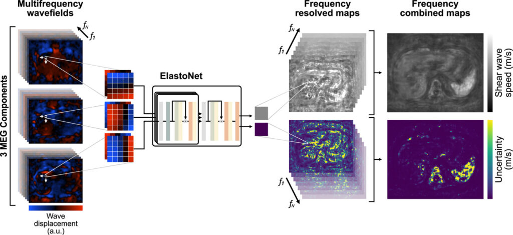
ElastoNet operates through a two-step hierarchical architecture:
- Wave Patch Embedding Block :
Each 5×5 pixel wave patch is passed through a convolutional layer followed by an attention mechanism. This helps the model learn spatial patterns and phase relationships within each patch. - Aggregation and Prediction Block :
After extracting features from all three motion-encoding gradient (MEG) components, the model aggregates them into a unified representation and predicts the shear wave speed along with uncertainty estimates.
Uncertainty quantification is achieved via evidential deep learning , where the model outputs not just a point estimate but also confidence bounds around that prediction. This is particularly valuable in clinical settings where decision-making must account for variability and reliability.
Why ElastoNet Stands Out: Key Advantages
1. Superior Accuracy Across Frequencies and Resolutions
One of the major challenges in MRE is ensuring consistent results across different imaging resolutions and excitation frequencies. Traditional methods like Local Frequency Estimation (LFE) and k-MDEV often require parameter tuning when applied to new datasets.
ElastoNet eliminates this need by being inherently resolution- and frequency-independent . It learns to predict wavelength in pixel numbers, which is then converted to physical units (m/s) based on known parameters like image resolution and vibration frequency.
This adaptability means ElastoNet can be used across multiple organs and patient populations without retraining.
2. Real-Time Uncertainty Quantification
Most MRE inversion tools provide a single stiffness map without any indication of confidence levels. ElastoNet changes this paradigm by integrating epistemic uncertainty estimation into its predictions.
Using Deep Evidential Learning , the model provides four output parameters:
- γ = predicted shear wavelength
- ν = precision of mean
- α = shape of variance
- β = scale of variance
These values are used to compute the final Shear Wave Speed (SWS) and its associated standard deviation , giving clinicians a clear picture of where the model is confident and where results might be less reliable.
3. Simultaneous Multicomponent Inversion
Traditional approaches often process each MEG component separately and then average the results. This can lead to information loss and reduced accuracy.
ElastoNet processes all three MEG components simultaneously, allowing the model to learn their interdependencies and improve inversion stability. Studies show this leads to lower root mean square error (RMSE) , especially in low-frequency and long-wavelength scenarios.
4. Robustness to Noise and Variability
ElastoNet was trained on synthetically generated wavefields with varying SNR, amplitudes, and phases. This ensures the model performs consistently even in noisy environments — a common challenge in clinical MRE acquisitions.
Tests on phantom data, finite element simulations, and in vivo human abdominal scans confirmed ElastoNet’s robustness across diverse conditions.
ElastoNet vs. Other MRE Inversion Methods
| FEATURE | LFE | K-MDEV | TWENN | ELASTONET |
|---|---|---|---|---|
| Resolution independence | ❌ | ❌ | ❌ | ✅ |
| Multifrequency support | ❌ | ❌ | ❌ | ✅ |
| Uncertainty quantification | ❌ | ❌ | ❌ | ✅ |
| Simultaneous MEG inversion | ❌ | ❌ | ❌ | ✅ |
| Reconstruction time (in vivo) | 236s | 32s | 77s (GPU) | 41s (GPU) |
ElastoNet outperforms established methods like LFE , k-MDEV , and even the recent TWENN in both accuracy and efficiency.
Applications of ElastoNet in Clinical Practice
ElastoNet has been tested in several clinical and experimental setups:
1. Abdominal MRE in Healthy Volunteers (n=14)
In a prospective study, ElastoNet was used to analyze abdominal MRE data at excitation frequencies ranging from 20 Hz to 80 Hz — one of the widest ranges ever reported in literature.
Results showed:
- Clear distinction between liver and spleen stiffness
- Mean SWS of 1.42 ± 0.04 m/s for the liver
- Mean SWS of 1.86 ± 0.12 m/s for the spleen
These values align closely with those obtained using k-MDEV and are significantly more stable than those from LFE or TWENN.
2. Phantom and Finite Element Modeling (FEM) Validation
ElastoNet was evaluated on:
- A phantom dataset with cylindrical inclusions of varying stiffness
- A human abdomen FEM simulation
In both cases, ElastoNet demonstrated:
- Lower RMSE compared to other methods
- Better contrast between stiff and soft regions
- More accurate boundary delineation
These findings validate ElastoNet’s ability to generalize across both synthetic and real-world data.
Limitations and Challenges of ElastoNet
While ElastoNet represents a significant advancement, it is not without its limitations:
1. Dependence on Synthetic Training Data
Like many deep learning models, ElastoNet relies on synthetically generated training data . While this ensures flexibility, it may not fully capture the complexity of real-world biological tissues, especially in heterogeneous environments like tumors or fibrotic livers.
2. No Direct Mechanical Parameter Estimation
Currently, ElastoNet only reconstructs shear wave speed (SWS) . Future work could extend it to estimate other viscoelastic properties such as storage modulus , loss modulus , or penetration depth .
3. Interpretability Concerns
Although ElastoNet offers uncertainty maps, the inner workings of the neural network remain somewhat opaque. Clinicians may prefer more interpretable models unless rigorous validation and explainability tools are integrated.
Future Directions and Potential Improvements
1. Integration with Physics-Informed Neural Networks (PINNs)
Combining ElastoNet with PINNs could allow the model to better adhere to the laws of continuum mechanics, improving generalization and interpretability.
2. Extension to 3D and Dynamic MRE
While ElastoNet currently works on 2D slices, extending it to 3D volumes and dynamic sequences would enhance its utility in brain and cardiac MRE.
3. Real-Time Implementation on MRI Scanners
Deploying ElastoNet directly on MRI scanners or PACS systems could enable real-time feedback during MRE exams, streamlining diagnosis and treatment planning.
If you’re Interested in Brain Artery Analysis using advance methods, you may also find this article helpful: CROWN Challenge Breakthrough: 6 AI Solutions Transform Brain Artery Analysis (But Still Fall Short)
Conclusion: ElastoNet – A New Era in MRE Analysis
ElastoNet marks a turning point in how we approach MRE inversion. By combining deep learning , uncertainty quantification , and multifrequency analysis , it addresses many of the shortcomings of traditional methods. Its ability to deliver accurate, resolution-independent results with built-in confidence measures makes it a strong candidate for widespread adoption in clinical practice.
Whether you’re a radiologist interpreting liver stiffness or a researcher developing new MRE protocols, ElastoNet offers a compelling solution with tangible benefits.
Call to Action: Try ElastoNet Today!
Are you involved in medical imaging research or clinical diagnostics? Don’t miss the chance to explore ElastoNet for yourself.
👉 Visit https://bioqic-apps.charite.de to access ElastoNet and test it on your own MRE datasets.
👉 Paper Link: https://doi.org/10.1016/j.media.2025.103642
Need help implementing ElastoNet in your workflow or customizing it for specific applications?
📩 Contact our team today to discuss collaboration opportunities, technical integration, or customized training modules.
Let’s bring the future of medical imaging into your lab — together.
Frequently Asked Questions (FAQs)
Q1: What is ElastoNet used for?
A: ElastoNet is used for wave inversion in Magnetic Resonance Elastography (MRE). It generates shear wave speed maps and provides uncertainty quantification to assess prediction reliability.
Q2: Can ElastoNet be used for different organs?
A: Yes, ElastoNet is designed to be organ-agnostic. It has been tested on abdominal MRE data but can be adapted for brain, breast, and cardiac applications.
Q3: How does ElastoNet handle noise in MRE data?
A: ElastoNet was trained on synthetically generated data with varying SNR levels, making it robust to noise commonly found in clinical MRE scans.
Q4: Is ElastoNet available for public use?
A: Yes, ElastoNet will be publicly accessible on https://bioqic-apps.charite.de upon full publication.
Q5: Does ElastoNet require GPU processing?
A: While it can run on CPU, ElastoNet achieves optimal performance with GPU acceleration (e.g., NVIDIA A100).
Final Thoughts
ElastoNet is more than just another neural network — it’s a paradigm shift in how we analyze biomechanical data from MRE. With its combination of accuracy , robustness , and transparency , it sets a new standard for AI-driven medical imaging.
As machine learning continues to reshape healthcare, tools like ElastoNet will play a pivotal role in delivering faster, more reliable diagnoses — and ultimately, better patient outcomes.
Below is a complete implementation of the ElastoNet model based on the information provided in the research paper. This implementation includes data generation, neural network architecture, training, and inference components.
import numpy as np
import tensorflow as tf
from tensorflow.keras import layers, models, optimizers, losses
import matplotlib.pyplot as plt
from scipy.special import gamma as gamma_func
import os

# Set random seeds for reproducibility
np.random.seed(42)
tf.random.set_seed(42)

class ElastoNet:
    def __init__(self, patch_size=5, batch_size=2048, learning_rate=1e-4, lambda_reg=0.05):
        self.patch_size = patch_size
        self.batch_size = batch_size
        self.learning_rate = learning_rate
        self.lambda_reg = lambda_reg
        self.model = self.build_model()

    def build_model(self):
        # Input layer for a single 5x5 complex-valued patch
        inputs_real = layers.Input(shape=(self.patch_size, self.patch_size), name='input_real')
        inputs_imag = layers.Input(shape=(self.patch_size, self.patch_size), name='input_imag')

        # Stack real and imaginary parts to form a 2-channel input
        x = layers.Concatenate(axis=-1)([inputs_real[..., tf.newaxis], inputs_imag[..., tf.newaxis]])

        # Normalize by average modulus
        mod = tf.sqrt(tf.square(inputs_real) + tf.square(inputs_imag))
        avg_mod = tf.reduce_mean(mod, axis=[1, 2], keepdims=True)
        x_norm = x / (avg_mod[..., tf.newaxis] + 1e-8)  # Add small epsilon to avoid division by zero

        # Embedding block
        x = layers.Conv2D(64, 1, activation='relu')(x_norm)

        # Attention layer
        b, h, w, c = x.shape
        x_flat = layers.Reshape((h*w, c))(x)
        attn_output = layers.MultiHeadAttention(num_heads=8, key_dim=8)(x_flat, x_flat)
        x = layers.Reshape((h, w, c))(attn_output)
        x = layers.Add()([x, x_flat])
        x = layers.LayerNormalization()(x)

        # Feed-forward layers
        for _ in range(5):
            x = layers.Dense(64, activation='relu')(x)
            x = layers.Dense(64)(x)
            x = layers.Add()([x, x])
            x = layers.Activation('relu')(x)
            x = layers.LayerNormalization()(x)

        # Create model that outputs features for one patch
        patch_model = models.Model(inputs=[inputs_real, inputs_imag], outputs=x)

        # Inputs for all three MEG components
        megs_real = [layers.Input(shape=(None, None), name=f'meg_real_{i}') for i in range(3)]
        megs_imag = [layers.Input(shape=(None, None), name=f'meg_imag_{i}') for i in range(3)]

        # Process each MEG component through the shared patch model
        features = []
        for i in range(3):
            feat = patch_model([megs_real[i], megs_imag[i]])
            features.append(feat)

        # Concatenate features from all MEG components
        x = layers.Concatenate(axis=-1)(features)

        # Second attention layer across spatial dimensions
        b, h, w, c = x.shape
        x_flat = layers.Reshape((h*w, c))(x)
        attn_output = layers.MultiHeadAttention(num_heads=8, key_dim=8)(x_flat, x_flat)
        x = layers.Reshape((h, w, c))(attn_output)
        x = layers.Add()([x, x_flat])
        x = layers.LayerNormalization()(x)

        # Final feed-forward layers
        for _ in range(2):
            x = layers.Dense(128, activation='relu')(x)
            x = layers.Dense(128)(x)
            x = layers.Add()([x, x])
            x = layers.Activation('relu')(x)
            x = layers.LayerNormalization()(x)

        # Output layer - four parameters of evidential distribution
        outputs = layers.Dense(4)(x)

        # Create final model
        model_inputs = megs_real + megs_imag
        return models.Model(inputs=model_inputs, outputs=outputs)

    def evidential_loss(self, y_true, outputs):
        # Extract evidential parameters from outputs
        gamma, v, alpha, beta = tf.split(outputs, 4, axis=-1)

        # Ensure positive values using softplus
        v = tf.nn.softplus(v)
        alpha = tf.nn.softplus(alpha) + 1.0  # alpha > 1 for variance to be defined
        beta = tf.nn.softplus(beta)

        # Negative log likelihood loss
        omega = 2 * beta * (1 + v)
        delta = (y_true - gamma) ** 2
        nll = 0.5 * tf.math.log(np.pi * v) - alpha * tf.math.log(omega)
        nll += tf.math.lgamma(alpha) - tf.math.lgamma(alpha + 0.5)
        nll += (alpha + 0.5) * tf.math.log(delta * v + omega)

        # Regularization term
        reg = tf.abs(y_true - gamma) * (2 * v + alpha)

        # Combine losses
        total_loss = tf.reduce_mean(nll + self.lambda_reg * reg)
        return total_loss

    def train_step(self, real_patches, imag_patches, y_true):
        with tf.GradientTape() as tape:
            outputs = self.model([real_patches, imag_patches])
            loss = self.evidential_loss(y_true, outputs)

        gradients = tape.gradient(loss, self.model.trainable_variables)
        self.optimizer.apply_gradients(zip(gradients, self.model.trainable_variables))
        return loss

    def train(self, epochs=300000):
        self.optimizer = optimizers.Adam(learning_rate=self.learning_rate)

        for epoch in range(epochs):
            # Generate synthetic data on the fly
            real_patches, imag_patches, wavelengths = self.generate_batch()

            # Train on batch
            loss = self.train_step(real_patches, imag_patches, wavelengths)

            if epoch % 100 == 0:
                print(f"Epoch {epoch}, Loss: {loss.numpy()}")

            if epoch % 10000 == 0 and epoch > 0:
                # Save model checkpoint
                self.model.save_weights(f"elastonet_epoch_{epoch}.h5")

    def generate_wave_patch(self, params):
        """Generate a single wave patch based on given parameters"""
        (amp_shear, phase_shear, amp_comp, phase_comp,
         num_sources_shear, num_sources_comp, distance, angle_inplane,
         angle_outofplane, shear_wavelength, comp_wavelength,
         shear_penetration, comp_penetration, snr) = params

        # Convert angles to radians
        angle_inplane = np.deg2rad(angle_inplane)
        angle_outofplane = np.deg2rad(angle_outofplane)

        # Create coordinate grid
        x = np.arange(self.patch_size)
        y = np.arange(self.patch_size)
        X, Y = np.meshgrid(x, y)
        coords = np.stack([X, Y], axis=-1)

        # Calculate normal vector direction
        nx = np.sin(angle_outofplane) * np.cos(angle_inplane)
        ny = np.sin(angle_outofplane) * np.sin(angle_inplane)
        nz = np.cos(angle_outofplane)
        normal = np.array([nx, ny, nz])

        # Initialize wave field
        wave_real = np.zeros((self.patch_size, self.patch_size))
        wave_imag = np.zeros((self.patch_size, self.patch_size))

        # Add shear waves
        for _ in range(num_sources_shear):
            # Random position within patch
            source_x = np.random.randint(0, self.patch_size)
            source_y = np.random.randint(0, self.patch_size)

            # Calculate distance from source for each pixel
            dists = np.sqrt((X - source_x)**2 + (Y - source_y)**2)

            # Wave number
            k_shear = 2 * np.pi / shear_wavelength

            # Phase term
            phase_term = k_shear * dists

            # Amplitude decay
            amp_decay = np.exp(-dists / shear_penetration)

            # Combine into wave
            wave_component = amp_shear * amp_decay * np.exp(-1j * phase_term)
            wave_component *= np.exp(1j * phase_shear)

            wave_real += np.real(wave_component)
            wave_imag += np.imag(wave_component)

        # Add compression waves
        for _ in range(num_sources_comp):
            # Random position within patch
            source_x = np.random.randint(0, self.patch_size)
            source_y = np.random.randint(0, self.patch_size)

            # Calculate distance from source for each pixel
            dists = np.sqrt((X - source_x)**2 + (Y - source_y)**2)

            # Wave number
            k_comp = 2 * np.pi / comp_wavelength

            # Phase term
            phase_term = k_comp * dists

            # Amplitude decay
            amp_decay = np.exp(-dists / comp_penetration)

            # Combine into wave
            wave_component = amp_comp * amp_decay * np.exp(-1j * phase_term)
            wave_component *= np.exp(1j * phase_comp)

            wave_real += np.real(wave_component)
            wave_imag += np.imag(wave_component)

        # Add noise
        signal_power = np.var(wave_real) + np.var(wave_imag)
        noise_power = signal_power / (10 ** (snr / 10))
        noise_real = np.random.normal(0, np.sqrt(noise_power), wave_real.shape)
        noise_imag = np.random.normal(0, np.sqrt(noise_power), wave_imag.shape)

        wave_real += noise_real
        wave_imag += noise_imag

        return wave_real, wave_imag, shear_wavelength

    def generate_batch(self):
        """Generate a batch of synthetic wave patches"""
        # Define parameter ranges from Table 1 in the paper
        param_ranges = {
            'amp_shear': (1e-6, 1),
            'phase_shear': (0, 2*np.pi),
            'amp_comp': (1e-6, 1),
            'phase_comp': (0, 2*np.pi),
            'num_sources_shear': (1, 6),
            'num_sources_comp': (1, 6),
            'distance': (5, 100),
            'angle_inplane': (0, 360),
            'angle_outofplane': (0, 180),
            'shear_wavelength': (2.5, 120),
            'comp_wavelength': (5000, 200000),
            'shear_penetration': (2.5, 120),
            'comp_penetration': (5000, 200000),
            'snr': (0, 30)
        }

        # Generate random parameters for each sample in batch
        batch_params = []
        for _ in range(self.batch_size):
            params = {}
            for key, (min_val, max_val) in param_ranges.items():
                if key in ['num_sources_shear', 'num_sources_comp']:
                    params[key] = np.random.randint(min_val, max_val+1)
                else:
                    params[key] = np.random.uniform(min_val, max_val)
            batch_params.append(params)

        # Generate patches
        real_patches = np.zeros((self.batch_size, self.patch_size, self.patch_size, 3))
        imag_patches = np.zeros((self.batch_size, self.patch_size, self.patch_size, 3))
        wavelengths = np.zeros((self.batch_size, self.patch_size, self.patch_size))

        for i, params in enumerate(batch_params):
            for j in range(3):  # Three MEG components
                real, imag, wl = self.generate_wave_patch(params)
                real_patches[i, :, :, j] = real
                imag_patches[i, :, :, j] = imag
                wavelengths[i, :, :, j] = wl

        return real_patches, imag_patches, wavelengths

    def predict(self, real_patches, imag_patches):
        """Make predictions on new data"""
        outputs = self.model.predict([real_patches, imag_patches])
        gamma, v, alpha, beta = tf.split(outputs, 4, axis=-1)

        # Apply softplus to ensure positive values
        v = tf.nn.softplus(v)
        alpha = tf.nn.softplus(alpha) + 1.0
        beta = tf.nn.softplus(beta)

        # Calculate uncertainty
        epistemic_uncertainty = beta / (v * (alpha - 1))

        return gamma, epistemic_uncertainty

    def save_model(self, path):
        """Save model weights"""
        self.model.save_weights(path)

    def load_model(self, path):
        """Load model weights"""
        self.model.load_weights(path)

    def visualize_results(self, real_patches, imag_patches, true_wavelengths):
        """Visualize predictions vs ground truth"""
        pred_gamma, pred_uncertainty = self.predict(real_patches, imag_patches)

        # Plot example results
        plt.figure(figsize=(15, 5))

        # Plot true wavelengths
        plt.subplot(1, 3, 1)
        plt.imshow(true_wavelengths[0, :, :, 0], cmap='viridis')
        plt.title('True Wavelengths')
        plt.colorbar()

        # Plot predicted wavelengths
        plt.subplot(1, 3, 2)
        plt.imshow(pred_gamma[0, :, :, 0], cmap='viridis')
        plt.title('Predicted Wavelengths')
        plt.colorbar()

        # Plot uncertainty
        plt.subplot(1, 3, 3)
        plt.imshow(pred_uncertainty[0, :, :, 0], cmap='plasma')
        plt.title('Epistemic Uncertainty')
        plt.colorbar()

        plt.tight_layout()
        plt.show()

# Example usage
if __name__ == "__main__":
    # Initialize ElastoNet model
    elastonet = ElastoNet()

    # Print model summary
    elastonet.model.summary()

    # Train the model
    elastonet.train(epochs=100)  # For demonstration purposes; full training would require more epochs

    # Save final model
    elastonet.save_model("elastonet_final.h5")
Pingback: 3 Breakthroughs & 1 Warning: How Explainable AI SVIS-RULEX is Revolutionizing Medical Imaging (Finally!) - aitrendblend.com