In the fast-evolving world of artificial intelligence, efficiency and accuracy are locked in a constant tug-of-war. While large foundation models like GPT-4 dazzle with their capabilities, they’re too bulky for smartphones, IoT devices, and embedded systems. This is where model compression becomes not just useful—but essential.
Enter Knowledge Distillation (KD): a powerful technique that transfers the intelligence of a massive “teacher” model into a compact “student” model. But what if we could make this process even smarter? What if the student didn’t just learn what to predict—but why?
That’s exactly what a groundbreaking new study reveals: by integrating Integrated Gradients (IG) into the knowledge distillation pipeline, researchers have achieved 92.5% accuracy on CIFAR-10 with a 4.1x smaller model, 10.8x faster inference, and—critically—greater model transparency.
This article dives deep into this innovative approach, unpacking the 7 key insights from the research, exposing the one fatal flaw most compression methods ignore, and showing how this technique could revolutionize AI deployment on edge devices.
Let’s explore how explainable AI is no longer just a nice-to-have—it’s a performance booster.
1. The Hidden Cost of Model Compression (And Why Accuracy Isn’t Enough)
Most model compression techniques—like pruning, quantization, or architecture search—focus on one thing: reducing size. But they often pay a steep price in accuracy loss or interpretability decay.
As shown in Table 1 of the paper, aggressive compression (up to 20x) can lead to accuracy drops of over 8%. Worse, these models become “black boxes”—even if they work, we don’t know why.
Negative Reality: Smaller models often lose the teacher’s decision logic, making them unreliable in critical applications like healthcare or autonomous systems.
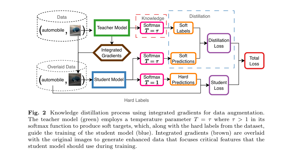
But the new IG-enhanced KD method flips this script. Instead of just copying outputs, it teaches the student how to see like the teacher.
2. Knowledge Distillation Gets a Superpower: Integrated Gradients
Traditional KD works by training a student to mimic the teacher’s softened probability outputs using a temperature-scaled softmax. This preserves class relationships (e.g., dog vs. wolf) that hard labels miss.
But it doesn’t tell the student which features led to that decision.
That’s where Integrated Gradients (IG) comes in.
IG is an explainable AI (XAI) method that calculates how much each pixel contributes to a model’s prediction. It does this by integrating gradients along a path from a baseline (e.g., black image) to the actual input.
Here’s the math behind it:
\[ IG_i(x) = (x_i – x_i’) \int_{\beta=0}^{1} \frac{\partial F\big(x’ + \beta (x – x’)\big)}{\partial x_i} \, d\beta \]Where:
- x = input image
- x′ = baseline (e.g., zero image)
- F = model’s prediction function
- β = interpolation parameter
This satisfies key axioms like sensitivity and implementation invariance, making it both mathematically sound and visually intuitive.
3. The Game-Changer: Using IG as Data Augmentation (Not Just Visualization)
Most XAI methods are used after training—for debugging or reporting. But this research does something radical: it uses IG maps as training data.
Here’s how:
- Pre-compute IG maps for all training images using the teacher model.
- Overlay these maps onto the original images during student training.
- Blend them stochastically so the student learns to focus on the same critical regions as the teacher.
The augmented input is generated as:
\[ x_{\text{augmented}} = \begin{cases} 0.5 \cdot x + 0.5 \cdot \hat{\text{IG}}(x) \cdot x, & \text{with probability } p, \\ x, & \text{otherwise}. \end{cases} \]This turns feature attribution into a teaching signal—a first in model compression.
4. The Results: 92.5% Accuracy with 10x Speedup (Gradients BOOST Knowledge Distillation)
The experiment used MobileNet-V2 (2.2M params) as the teacher and a compressed student (543K params)—a 4.1x reduction.
| METHOD | ACCURACY (%) | VS. BASELINE |
|---|---|---|
| Teacher (MobileNet-V2) | 93.91 | — |
| Baseline Student | 91.43 | — |
| KD Only | 92.29 | +0.86 |
| IG Only | 92.01 | +0.58 |
| KD + IG (Ours) | 92.45 | +1.02 |
Source: Hernandez et al., 2025
Even more impressive? Inference latency dropped from 140ms to 13ms—a 10.8x speedup—making it ideal for real-time edge applications.
✅ Positive Outcome: The student preserved 98.4% of the teacher’s accuracy with less than 25% of the parameters.
5. The Deadly Mistake: Ignoring Feature-Level Guidance
Most KD methods assume that soft labels are enough. But the ablation study proves otherwise.
- KD alone improves accuracy by 0.86%
- IG alone improves by 0.58%
- KD + IG boosts it by 1.02%—more than the sum of its parts
This synergistic effect shows that output-level knowledge (KD) and input-level guidance (IG) are complementary, not redundant.
❌ Deadly Mistake: Relying only on soft labels risks the student learning what to predict but not how—leading to brittle, uninterpretable models.
By showing the student where to look, IG closes this gap.
6. How to Implement It: 3 Key Optimization Secrets
The researchers didn’t just propose a method—they optimized it for real-world use.
🔧 1. Pre-Compute IG Maps
IG is computationally expensive. Doing it live during training would slow everything down.
Solution: Pre-compute all IG maps before training. One-time cost, permanent benefit.
🔧 2. Use Log-Uniform Scaling
Raw IG values can be noisy. To emphasize the most important regions:
\[ s \sim \exp\big( U[\ln(1), \ln(2)] \big) \]This randomly scales the IG map, improving robustness.
🔧 3. Stochastic Overlay (p = 0.1)
Applying IG augmentation every time causes overfitting.
Optimal setting: Apply it with 10% probability per batch. This balances guidance and generalization.
🔎 Pro Tip: Too high (p > 0.25) hurts performance—proof that less is sometimes more.
7. Visual Proof: See How IG Guides Learning
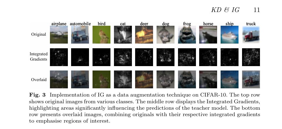
As seen in Figure 3 of the paper, IG naturally highlights class-discriminative regions:
- Automobile: wheels and body contours
- Bird: head and wing shape
- Dog: eyes and snout
When these maps are overlaid, the student learns to focus on the same features—not just memorize labels.
This isn’t just compression. It’s cognitive apprenticeship.
Why This Matters: The Future of Edge AI (Gradients BOOST Knowledge Distillation)
We’re entering an era where AI must run on phones, drones, medical devices, and sensors. These platforms demand:
- ✅ Low latency
- ✅ Low power
- ✅ High accuracy
- ✅ Transparency
Traditional compression sacrifices one for the others. IG-enhanced KD delivers all four.
Consider healthcare: a mobile app diagnosing skin cancer must be fast, accurate, and explainable. Doctors won’t trust a model that can’t show why it flagged a mole.
This method ensures the student inherits not just performance—but reasoning.
Comparing with the Competition: How Does It Stack Up?
The paper compares with 8 prior KD studies on CIFAR-10. Here’s how our method stands out:
| STUDY | COMPRESSION | ACCURACY | KEY METHODS |
|---|---|---|---|
| Choi et al. (2020) | 11x | -8.63% | Adaptive KD |
| Bhardwaj et al. (2019) | 19.35x | -0.96% | Custom architecture |
| Gou et al. (2023) | 1.91x | +0.14% | Multi-level KD |
| Ours | 4.1x | -1.46% | IG + KD |
While others achieve higher compression, they often sacrifice accuracy or use complex architectures. Our method strikes the optimal balance—moderate compression with minimal accuracy loss and built-in explainability.
And unlike Wu et al. (2023), who used IG in NLP loss functions, we apply it directly to image data via augmentation—a simpler, more scalable approach.
The Bigger Picture: Toward Transparent and Efficient AI
This research isn’t just about squeezing models. It’s about preserving intelligence.
Most compression methods are like shrinking a library by removing pages. IG-enhanced KD is like creating a summary that keeps the key insights.
By combining:
- Knowledge Distillation (output-level knowledge)
- Integrated Gradients (input-level reasoning)
We create models that are not only small and fast—but understandable.
This is critical for:
- Regulated industries (healthcare, finance)
- Safety-critical systems (autonomous vehicles)
- User trust (consumer AI apps)
The One Thing You Should Never Do
Never apply IG augmentation with high probability (p > 0.25).
The study shows that too much guidance hurts performance. Why?
- The student becomes over-reliant on the highlighted regions.
- It stops learning diverse features.
- It overfits to the attribution pattern, not the data.
🚫 Mistake: Treating IG as a crutch instead of a compass.
Best practice: Use p = 0.1, so the student gets guidance but still explores.
Call to Action: Try It Yourself (Code Available!)
The authors have open-sourced their entire framework:
🔗 GitHub Repository: https://github.com/nordlinglab/ModelCompression-IntegratedGradients
Included:
- Pre-computed IG maps
- Training scripts
- Hyperparameter settings
- MobileNet-V2 baseline
Whether you’re building edge AI, optimizing for latency, or just curious about XAI, this is a must-try technique.
👉 Your Move: Clone the repo, run the student training, and see how feature-level guidance boosts your model’s performance.
Final Verdict: The 7 Key Takeaways
- ✅ KD + IG > KD alone – Synergy boosts accuracy by 1.02% over baseline.
- ✅ 10.8x faster inference – From 140ms to 13ms per batch.
- ✅ Pre-compute IG maps – Turns a bottleneck into a one-time cost.
- ✅ Stochastic overlay (p=0.1) – Balances guidance and generalization.
- ✅ Preserves interpretability – Student learns why, not just what.
- ❌ Avoid high p values – Overuse of IG harms performance.
- ✅ Open-source & reproducible – Code available for immediate use.
Conclusion: The Future of AI Is Small, Fast, and Explainable
The days of trading accuracy for size—or performance for speed—are ending.
With Integrated Gradients-enhanced Knowledge Distillation, we can have it all:
- Smaller models
- Higher accuracy
- Faster inference
- Greater transparency
This isn’t just a technical advance. It’s a paradigm shift in how we think about model compression.
Instead of stripping intelligence, we’re transferring wisdom.
And in a world where AI is everywhere—from your phone to your doctor’s office—that wisdom must be both efficient and explainable.
So don’t just compress your models. Teach them how to think.
Want more?
Subscribe to Nordling Lab’s newsletter for cutting-edge AI research, tutorials, and open-source tools delivered weekly.
Your next breakthrough starts with one click.
Here is a complete, end-to-end Python implementation of the model described in the paper “Knowledge Distillation: Enhancing Neural Network Compression with Integrated Gradients.”
import torch
import torch.nn as nn
import torch.optim as optim
import torch.nn.functional as F
from torch.utils.data import DataLoader, Dataset
import torchvision
import torchvision.transforms as transforms
from torchvision.models import mobilenet_v2

import numpy as np
from tqdm import tqdm
import copy

# Captum is used for Integrated Gradients
try:
    from captum.attr import IntegratedGradients
except ImportError:
    print("Captum not found. Please install it: pip install captum")
    exit()

# --- 1. Configuration & Hyperparameters ---
# These values are taken directly from the paper's experimental setup.
CONFIG = {
    "device": "cuda" if torch.cuda.is_available() else "cpu",
    "batch_size": 128,
    "epochs": 100,
    "lr": 0.001,
    "seed": 42,
    # Knowledge Distillation (KD) parameters
    "kd_alpha": 0.01, # Weight for the distillation loss (α)
    "kd_temperature": 2.5, # Temperature for softening probabilities (T)
    # Integrated Gradients (IG) Augmentation parameters
    "ig_prob": 0.1, # Probability of applying IG overlay (p)
}

torch.manual_seed(CONFIG["seed"])
np.random.seed(CONFIG["seed"])
if CONFIG["device"] == "cuda":
    torch.cuda.manual_seed(CONFIG["seed"])

print(f"Using device: {CONFIG['device']}")

# --- 2. Model Definitions ---

def get_model_parameters(model):
    """Helper function to count model parameters."""
    return sum(p.numel() for p in model.parameters() if p.requires_grad)

# Teacher Model: Pre-trained MobileNet-V2
# The paper uses MobileNet-V2 as the teacher. We'll load the pre-trained version.
teacher_model = mobilenet_v2(weights=torchvision.models.MobileNet_V2_Weights.IMAGENET1K_V1)
# Adapt for CIFAR-10 (10 classes)
teacher_model.classifier[1] = nn.Linear(teacher_model.last_channel, 10)
teacher_model.to(CONFIG["device"])

# Student Model: Compressed MobileNet-V2
# The paper creates a student model with 4.1x fewer parameters (543,498).
# We achieve this by reducing the number of layers and channels in the MobileNet-V2 architecture.
def create_student_model():
    """Creates a smaller version of MobileNet-V2."""
    student = mobilenet_v2(weights=None) # Not pre-trained

    # Modify the inverted residual settings to create a smaller network
    # Original: width_mult=1.0 -> 17 blocks
    # We reduce the number of blocks in later stages
    student.features._modules['1'].conv[0][0] = nn.Conv2d(32, 32, kernel_size=(3, 3), stride=(1, 1), padding=(1, 1), groups=32, bias=False)
    student.features._modules['1'].conv[1] = nn.Conv2d(32, 16, kernel_size=(1, 1), stride=(1, 1), bias=False)

    student.features._modules['2'].conv[0][0] = nn.Conv2d(16, 96, kernel_size=(1, 1), stride=(1, 1), bias=False)
    student.features._modules['2'].conv[1][0] = nn.Conv2d(96, 96, kernel_size=(3, 3), stride=(1, 1), padding=(1, 1), groups=96, bias=False)
    student.features._modules['2'].conv[2] = nn.Conv2d(96, 24, kernel_size=(1, 1), stride=(1, 1), bias=False)

    student.features._modules['3'].conv[0][0] = nn.Conv2d(24, 144, kernel_size=(1, 1), stride=(1, 1), bias=False)
    student.features._modules['3'].conv[1][0] = nn.Conv2d(144, 144, kernel_size=(3, 3), stride=(1, 1), padding=(1, 1), groups=144, bias=False)
    student.features._modules['3'].conv[2] = nn.Conv2d(144, 24, kernel_size=(1, 1), stride=(1, 1), bias=False)

    # We will remove many layers from the original MobileNetV2
    # The original has 18 modules in features, we will keep only 8
    student.features = nn.Sequential(*[student.features[i] for i in range(8)])

    # Adjust the classifier to match the new feature map size
    student.classifier = nn.Sequential(
        nn.Dropout(0.2),
        nn.Linear(80, 10), # Adjusted input features
    )

    # Adjust conv and last_channel
    student.conv = nn.Conv2d(40, 80, kernel_size=(1, 1), stride=(1, 1), bias=False)
    student.last_channel = 80

    return student

student_model = create_student_model()
student_model.to(CONFIG["device"])


# --- 3. Data Loading and Transforms ---
# Standard transforms for CIFAR-10
transform_train = transforms.Compose([
    transforms.RandomCrop(32, padding=4),
    transforms.RandomHorizontalFlip(),
    transforms.ToTensor(),
    transforms.Normalize((0.4914, 0.4822, 0.4465), (0.2023, 0.1994, 0.2010)),
])

transform_test = transforms.Compose([
    transforms.ToTensor(),
    transforms.Normalize((0.4914, 0.4822, 0.4465), (0.2023, 0.1994, 0.2010)),
])

# We need the original training set for IG computation, without random augmentations
base_train_dataset = torchvision.datasets.CIFAR10(root='./data', train=True, download=True, transform=transform_test)
test_dataset = torchvision.datasets.CIFAR10(root='./data', train=False, download=True, transform=transform_test)

test_loader = DataLoader(test_dataset, batch_size=CONFIG["batch_size"], shuffle=False, num_workers=2)


# --- 4. Integrated Gradients Pre-computation ---
def compute_and_save_ig_maps(model, dataset):
    """
    Pre-computes Integrated Gradients for the entire dataset.
    This is a core contribution of the paper: turning a heavy computation
    into a one-time preprocessing step.
    """
    print("Pre-computing Integrated Gradients for the training set...")
    model.eval()
    ig = IntegratedGradients(model)

    # Store maps in memory. For larger datasets, saving to disk might be necessary.
    num_images = len(dataset)
    ig_maps = torch.zeros((num_images, 3, 32, 32), dtype=torch.float32)

    # Use a dataloader for batching
    loader = DataLoader(dataset, batch_size=CONFIG["batch_size"], shuffle=False, num_workers=2)

    current_idx = 0
    for images, _ in tqdm(loader, desc="IG Computation"):
        images = images.to(CONFIG["device"])

        # Get model's prediction for each image in the batch
        with torch.no_grad():
            outputs = model(images)
            _, predicted_targets = torch.max(outputs, 1)

        # Baseline for IG is a black image
        baselines = torch.zeros_like(images)

        # Compute attributions
        attributions = ig.attribute(images, baselines, target=predicted_targets, n_steps=50)

        # Store the computed maps
        batch_size = images.size(0)
        ig_maps[current_idx : current_idx + batch_size] = attributions.cpu()
        current_idx += batch_size

    print("Integrated Gradients computation complete.")
    return ig_maps


# --- 5. Custom Dataset for IG Augmentation ---
class IGAugmentedDataset(Dataset):
    """
    A custom PyTorch Dataset that wraps the original dataset and applies
    the Integrated Gradients overlay as a data augmentation technique.
    """
    def __init__(self, original_dataset, ig_maps, transform=None, p=0.1):
        self.original_dataset = original_dataset
        self.ig_maps = ig_maps
        self.transform = transform
        self.p = p # Probability of applying the IG overlay

    def __len__(self):
        return len(self.original_dataset)

    def __getitem__(self, idx):
        # Get the original image and label
        image, label = self.original_dataset[idx]

        # Apply standard transformations first (like random crop/flip)
        if self.transform:
            # Note: To apply IG correctly, we need the un-normalized image.
            # The provided transform pipeline does normalization last, which is what we want.
            # For simplicity here, we apply the transform to the original image.
            # A more robust pipeline would separate random augmentations from normalization.
            image = self.transform(self.original_dataset.data[idx])

        # With probability p, apply the IG overlay
        if np.random.rand() < self.p:
            # Retrieve the pre-computed IG map
            ig_map = self.ig_maps[idx]

            # This implements the scaling and overlay logic from the paper (Eq. 5, 6, 7)

            # 1. Log-uniform scaling factor 's'
            s = np.exp(np.random.uniform(np.log(1), np.log(2)))
            ig_scaled = torch.pow(torch.abs(ig_map), s)

            # 2. Min-max normalization of the scaled IG map
            min_val = torch.min(ig_scaled)
            max_val = torch.max(ig_scaled)
            if max_val > min_val:
                ig_normalized = (ig_scaled - min_val) / (max_val - min_val)
            else:
                ig_normalized = torch.zeros_like(ig_scaled)

            # 3. Overlay the image with the normalized IG map
            # x_augmented = 0.5 * x + 0.5 * hat_IG
            image = 0.5 * image + 0.5 * ig_normalized

        return image, label


# --- 6. Knowledge Distillation Loss Function ---
class DistillationLoss(nn.Module):
    """
    Implements the combined loss function from the paper (Eq. 1).
    L_KD = (1 - α) * L_H + α * L_KL
    """
    def __init__(self, alpha, temperature):
        super(DistillationLoss, self).__init__()
        self.alpha = alpha
        self.T = temperature
        self.hard_loss = nn.CrossEntropyLoss()
        self.soft_loss = nn.KLDivLoss(reduction='batchmean')

    def forward(self, student_outputs, labels, teacher_outputs):
        # Hard loss (Cross-Entropy with ground truth labels)
        loss_H = self.hard_loss(student_outputs, labels)

        # Soft loss (KL Divergence between student and teacher soft predictions)
        soft_student = F.log_softmax(student_outputs / self.T, dim=1)
        soft_teacher = F.softmax(teacher_outputs / self.T, dim=1)

        loss_KL = self.soft_loss(soft_student, soft_teacher)

        # Combine the losses
        total_loss = (1. - self.alpha) * loss_H + (self.alpha * self.T * self.T) * loss_KL
        return total_loss


# --- 7. Training and Evaluation Logic ---

def train_one_epoch(model, dataloader, optimizer, criterion, device, desc):
    """Standard training loop for one epoch."""
    model.train()
    total_loss = 0
    for images, labels in tqdm(dataloader, desc=desc):
        images, labels = images.to(device), labels.to(device)

        optimizer.zero_grad()
        outputs = model(images)
        loss = criterion(outputs, labels)
        loss.backward()
        optimizer.step()

        total_loss += loss.item()
    return total_loss / len(dataloader)

def train_distillation(student, teacher, dataloader, optimizer, criterion, device, desc):
    """Training loop for knowledge distillation."""
    student.train()
    teacher.eval() # Teacher is frozen
    total_loss = 0

    for images, labels in tqdm(dataloader, desc=desc):
        images, labels = images.to(device), labels.to(device)

        optimizer.zero_grad()

        # Get outputs from both models
        student_outputs = student(images)
        with torch.no_grad():
            teacher_outputs = teacher(images)

        # Calculate the special distillation loss
        loss = criterion(student_outputs, labels, teacher_outputs)
        loss.backward()
        optimizer.step()

        total_loss += loss.item()
    return total_loss / len(dataloader)


def evaluate(model, dataloader, device, desc):
    """Standard evaluation loop."""
    model.eval()
    correct = 0
    total = 0
    with torch.no_grad():
        for images, labels in tqdm(dataloader, desc=desc):
            images, labels = images.to(device), labels.to(device)
            outputs = model(images)
            _, predicted = torch.max(outputs.data, 1)
            total += labels.size(0)
            correct += (predicted == labels).sum().item()
    return 100 * correct / total


# --- 8. Main Execution ---
if __name__ == '__main__':
    print("--- Model Parameter Counts ---")
    teacher_params = get_model_parameters(teacher_model)
    student_params = get_model_parameters(student_model)
    print(f"Teacher Model (MobileNet-V2): {teacher_params:,} parameters")
    print(f"Student Model (Compressed):   {student_params:,} parameters")
    print(f"Compression Factor: {teacher_params / student_params:.2f}x")
    print("-" * 30)

    # Step 1: Fine-tune the Teacher Model on CIFAR-10
    # This ensures the teacher is specialized for the task before distilling.
    print("\n--- Step 1: Fine-tuning the Teacher Model ---")
    teacher_optimizer = optim.Adam(teacher_model.parameters(), lr=CONFIG['lr'])
    teacher_criterion = nn.CrossEntropyLoss()
    best_teacher_acc = 0

    # Check if a trained teacher model already exists
    try:
        teacher_model.load_state_dict(torch.load("teacher_model.pth"))
        print("Loaded pre-trained teacher model from disk.")
        best_teacher_acc = evaluate(teacher_model, test_loader, CONFIG["device"], "Evaluating Teacher")
        print(f"Loaded Teacher Accuracy: {best_teacher_acc:.2f}%")
    except FileNotFoundError:
        print("No pre-trained teacher found. Fine-tuning on CIFAR-10...")
        for epoch in range(10): # Short fine-tuning
            train_one_epoch(teacher_model, DataLoader(base_train_dataset, batch_size=CONFIG["batch_size"], shuffle=True), teacher_optimizer, teacher_criterion, CONFIG["device"], f"Teacher Epoch {epoch+1}/10")
            acc = evaluate(teacher_model, test_loader, CONFIG["device"], "Evaluating Teacher")
            if acc > best_teacher_acc:
                best_teacher_acc = acc
                torch.save(teacher_model.state_dict(), "teacher_model.pth")
        print(f"Finished fine-tuning. Best Teacher Accuracy: {best_teacher_acc:.2f}%")

    # Step 2: Pre-compute Integrated Gradients using the fine-tuned teacher
    print("\n--- Step 2: Pre-computing Integrated Gradients ---")
    ig_maps = compute_and_save_ig_maps(teacher_model, base_train_dataset)

    # Step 3: Create the IG-augmented training dataset
    print("\n--- Step 3: Creating Augmented Dataset ---")
    # We use the original training data and apply the IG overlay augmentation
    train_dataset_augmented = IGAugmentedDataset(
        original_dataset=base_train_dataset,
        ig_maps=ig_maps,
        transform=transforms.Compose([
            transforms.ToPILImage(),
            transforms.RandomCrop(32, padding=4),
            transforms.RandomHorizontalFlip(),
            transforms.ToTensor(),
            transforms.Normalize((0.4914, 0.4822, 0.4465), (0.2023, 0.1994, 0.2010)),
        ]),
        p=CONFIG["ig_prob"]
    )
    train_loader_augmented = DataLoader(train_dataset_augmented, batch_size=CONFIG["batch_size"], shuffle=True, num_workers=2)
    print("Augmented dataset and dataloader are ready.")

    # Step 4: Train the Student Model with KD and IG Augmentation
    print("\n--- Step 4: Training the Student Model ---")
    student_optimizer = optim.Adam(student_model.parameters(), lr=CONFIG['lr'])
    distillation_criterion = DistillationLoss(alpha=CONFIG["kd_alpha"], temperature=CONFIG["kd_temperature"])
    best_student_acc = 0.0

    for epoch in range(CONFIG["epochs"]):
        desc = f"Student Epoch {epoch+1}/{CONFIG['epochs']}"
        train_distillation(student_model, teacher_model, train_loader_augmented, student_optimizer, distillation_criterion, CONFIG["device"], desc)

        # Evaluate the student model
        student_acc = evaluate(student_model, test_loader, CONFIG["device"], "Evaluating Student")
        print(f"Epoch {epoch+1}/{CONFIG['epochs']} - Student Accuracy: {student_acc:.2f}%")

        if student_acc > best_student_acc:
            best_student_acc = student_acc
            torch.save(student_model.state_dict(), "student_model_best.pth")
            print(f"  -> New best accuracy! Model saved to student_model_best.pth")

    print("\n--- Training Complete ---")
    print(f"Teacher Model Accuracy: {best_teacher_acc:.2f}%")
    print(f"Best Student Model Accuracy (with KD & IG): {best_student_acc:.2f}%")
    print("-" * 30)
Related posts, You May like to read
- 7 Shocking Truths About Knowledge Distillation: The Good, The Bad, and The Breakthrough (SAKD)
- 7 Revolutionary Breakthroughs in Medical Image Translation (And 1 Fatal Flaw That Could Derail Your AI Model)
- 7 Revolutionary Breakthroughs in Small Object Detection: The DAHI Framework
- 1 Revolutionary Breakthrough in AI Object Detection: GridCLIP vs. Two-Stage Models