In the world of digital imaging, capturing clear, vibrant photos in low-light conditions has always been a challenge. From dimly lit cityscapes to indoor environments with minimal lighting, traditional cameras and enhancement algorithms often fail to preserve detail, color accuracy, and structural integrity. Enter ISALUX — a groundbreaking deep learning framework that redefines low-light image enhancement (LLIE) by integrating illumination priors, semantic segmentation maps, and a Mixture of Experts (MoE)-based architecture within a Vision Transformer (ViT) backbone.
Published in August 2025, the paper “ISALUX: Illumination and Semantics-Aware Transformer Employing Mixture of Experts for Low Light Image Enhancement“ introduces a novel approach that not only outperforms existing state-of-the-art methods but does so with remarkable computational efficiency.
In this article, we’ll dive deep into how ISALUX works, why it’s a game-changer for computer vision, and what makes it stand out in the crowded field of image enhancement technologies.
What Is Low-Light Image Enhancement?
Low-light image enhancement (LLIE) refers to the process of improving the visual quality of images captured under poor lighting conditions. These images typically suffer from:
- High noise levels
- Poor contrast and visibility
- Color distortion
- Loss of fine details
Traditional solutions like histogram equalization or Retinex-based models have limitations in preserving naturalness and avoiding artifacts. With the rise of deep learning, convolutional neural networks (CNNs) improved performance, but they struggle with long-range dependencies — crucial for understanding global scene structure.
Enter Vision Transformers (ViTs), which use self-attention mechanisms to capture contextual relationships across the entire image. However, most ViT-based LLIE models treat all pixels uniformly, ignoring semantic meaning and regional illumination variations.
ISALUX solves this by fusing illumination awareness and semantic understanding directly into its attention mechanism.
Introducing ISALUX: The Core Innovations
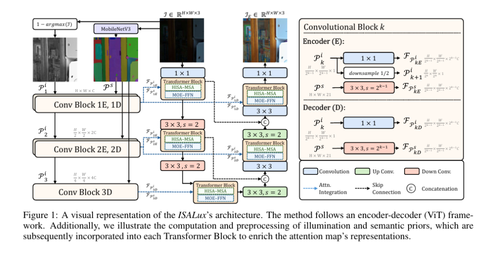
ISALUX stands for Illumination and Semantics-Aware Transformer with Mixture of Experts for Low-Light Image Enhancement. It’s built on a U-shaped encoder-decoder ViT architecture and introduces three key innovations:
- Hybrid Illumination and Semantics-Aware Multi-Headed Self-Attention (HISA-MSA)
- Mixture of Experts Feed-Forward Network (MoE-FFN)
- Low-Rank Adaptation (LoRA) for Regularization
Let’s explore each in detail.
1. HISA-MSA: Attention That Understands Light and Meaning
The heart of ISALUX is the HISA-MSA block, a custom self-attention module that integrates two types of priors:
🔹 Illumination Prior
The illumination prior helps the model understand the distribution of light across the image. It is computed as:
\[ P_i = 1 – \arg\max(I), \quad P_i \in \mathbb{R}^{H \times W \times 1} \]where I is the input image and argmaxc returns the maximum channel value per pixel (approximating brightness).
This prior is then downsampled into a pyramid: Pi0, Pi1, Pi2 , matching the spatial resolution at different network stages.
🔹 Semantic Prior
Semantic segmentation provides structural context — knowing what objects are in the scene (e.g., sky, person, car) allows region-specific enhancement. ISALUX uses MobileNetV3 as a lightweight segmentation backbone trained on COCO, producing a 21-channel probability map:
\[ P_s = \text{MobileNetV3}(I), \quad P_s \in \mathbb{R}^{H \times W \times 21} \]These priors are fused into the self-attention process via two parallel attention streams:
- One focuses on illumination-aware features
- The other on semantics-aware features
The final attention map is a weighted combination:
\[ ME = \nu \cdot (M_i \odot FP_i) + \omega \cdot (M_s \odot FP_s) \]where Mi and Ms are attention outputs modulated by illumination and semantic maps, and υ , ω are learnable weights.
This hybrid design ensures that dark regions are brightened intelligently, while edges and object boundaries remain sharp and artifact-free.
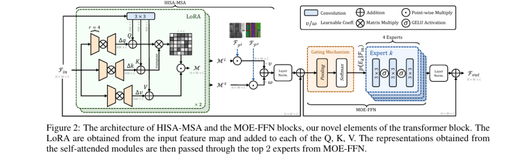
2. MoE-FFN: Specialized Processing with Dynamic Expert Selection
After attention, features pass through a Mixture of Experts Feed-Forward Network (MoE-FFN) — a sparse, adaptive layer that activates only the most relevant “experts” based on input content.
Each expert is a small CNN stack:
\[ E_i(F_{\text{in}}) = \text{Conv}_{1\times1}\Big(\sigma\big(\text{Conv}_{3\times3}(\sigma(\text{Conv}_{1\times1}(F_{\text{in}})))\big)\Big) \]where σ is the GELU activation.
A gating mechanism computes selection probabilities:
\[ G = \text{softmax}\!\left(W_g \cdot \text{avg_pool}(F’_{\text{in}})\right), \quad G \in \mathbb{R}^N \]Then, only the top-K experts (K=2 in ISALUX) are activated:
\[ F_{\text{out}} = \sum_{i=1}^{K} p(E_i \mid F_{\text{in}}’) \cdot E_i(F_{\text{in}}’) \]This design enables:
- Efficient computation (only 2/4 experts active)
- Specialized processing (e.g., one expert handles shadows, another reduces noise)
- Adaptability to diverse lighting scenarios
Compared to dense FFNs, MoE improves performance without bloating parameters.
3. LoRA: Preventing Overfitting with Low-Rank Adaptations
To prevent overfitting caused by unique lighting patterns in training data, ISALUX enhances the attention projections (Q, K, V) with Low-Rank Adaptations (LoRA).
Instead of updating full weight matrices, LoRA adds trainable low-rank matrices:
\[ \Delta q = \big(F_{\text{in}}’ \cdot \alpha_q \big) \cdot \beta_q, \quad \alpha_q \in \mathbb{R}^{C \times \tfrac{C}{r}}, \; \beta_q \in \mathbb{R}^{\tfrac{C}{r} \times C} \]These are added to the original queries, keys, and values:
\[ Q = Q_{0} + \Delta q, \quad K = K_{0} + \Delta k, \quad V = V_{0} + \Delta v \]
Benefits:
- Parameter efficiency (adds only ~0.1% extra params)
- Regularization against dataset-specific lighting biases
- Faster convergence during training
This makes ISALUX more robust when deployed in real-world, unseen environments.
Performance: How Does ISALUX Compare?
ISALUX was evaluated across multiple benchmarks, including LOL-v1, LOL-v2, SDSD, and LOL-Blur. Results show it consistently outperforms state-of-the-art models.
📊 Quantitative Results on LOL & SDSD Datasets
| METHOD | Params (M) | Avg PSNR ↑ | Avg SSIM ↑ |
|---|---|---|---|
| Restormer [41] | 26.1 | 22.85 | 0.822 |
| Retinexformer [25] | 1.61 | 28.71 | 0.884 |
| GLARE [44] | 44.04 | 29.42 | 0.905 |
| ISALUX (Ours) | 1.85 | 30.08 | 0.910 |
✅ ISALUX achieves the highest average PSNR (30.08 dB) and SSIM (0.910)
✅ 96% more parameter-efficient than GLARE
✅ Outperforms Retinexformer by +1.37 dB PSNR
🌟 No-Reference Evaluation (NIQE)
On datasets without ground truth (MEF, LIME, DICM, NPE), ISALUX achieves the lowest NIQE score (3.34), indicating superior perceptual quality.
| MEF | LIME | DICM | NPE | Avg NIQE ↓ | |
|---|---|---|---|---|---|
| GLARE [44] | 3.66 | 4.52 | 3.61 | 4.19 | 3.99 |
| ISALUX (Ours) | 3.58 | 3.91 | 3.21 | 3.40 | 3.34 |
Lower NIQE = more natural-looking images. ISALUX excels in color fidelity and illumination consistency.
⚡ Inference Speed: Real-Time Ready
Despite its advanced architecture, ISALUX is incredibly fast:
| MODEL | INFERENCE TIME (400 x 600) |
|---|---|
| Retinexformer | 300 ms |
| LLFlow | 378 ms |
| GLARE | 650 ms |
| ISALUX | 105 ms |
At 105 milliseconds per image, ISALUX is ideal for real-time applications like surveillance, autonomous driving, and mobile photography.
Ablation Study: What Really Makes ISALUX Work?
The authors conducted ablation studies to validate each component:
🔬 Effect of Priors
| CONFIGURATION | PSNR | SSIM |
|---|---|---|
| No Priors | 27.04 | 0.870 |
| + Illumination Prior | 27.15 | 0.878 |
| + Semantic Prior | 27.36 | 0.879 |
| + Both Priors (no LoRA) | 27.41 | 0.880 |
| Full ISALUX (with LoRA) | 27.63 | 0.881 |
➡️ Semantic prior contributes more than illumination (+0.32 dB vs +0.11 dB)
➡️ Combining both gives +0.59 dB improvement
➡️ LoRA adds final 0.22 dB boost
🧪 Loss Function Analysis
ISALUX uses a hybrid loss:
\[ L = \lambda_{1} L_{2} + \lambda_{2} L_{\text{perc}} + \lambda_{3} L_{\text{SSIM}} \]where:
- L2 : MSE for pixel accuracy
- Lperc : VGG-19 based perceptual loss
- LSSIM : Multi-scale structural similarity
Results show:
- L2 alone → 26.95 dB
- L2 + VGG19 → 27.08 dB (+0.13 dB)
- L2 + VGG19 + MS-SSIM → 27.63 dB (+0.55 dB)
This confirms that perceptual and structural losses are critical for high-quality enhancement.
Why ISALUX Matters: Real-World Applications
ISALUX isn’t just a research breakthrough — it has practical implications across industries:
📸 Photography & Mobile Imaging
Smartphones can leverage ISALUX to enhance night-mode photos with better detail, natural colors, and less noise, all while running efficiently on-device.
🚗 Autonomous Vehicles
Self-driving cars rely on clear vision in low-light conditions. ISALUX can improve object detection and depth estimation in tunnels, night driving, or foggy environments.
🏥 Medical Imaging
Low-dose X-rays or endoscopic videos often suffer from poor illumination. ISALUX can enhance visibility without introducing artifacts.
🕵️ Surveillance & Security
CCTV footage from poorly lit areas can be enhanced for facial recognition or activity analysis, improving public safety.
How to Use ISALUX (Coming Soon)
The authors plan to release the code upon publication, making ISALUX accessible to researchers and developers. Based on the architecture, it will likely be implemented in PyTorch with support for:
- Pretrained weights on LOL and SDSD datasets
- Semantic segmentation backbone (MobileNetV3)
- Configurable MoE and LoRA settings
Potential integration paths:
- As a standalone enhancement tool
- Embedded in larger vision pipelines (e.g., object detection)
- Adapted for video enhancement (via temporal priors)
Conclusion: The Future of Low-Light Enhancement Is Here
ISALUX represents a paradigm shift in low-light image enhancement. By combining:
✅ Illumination-aware attention
✅ Semantic-guided enhancement
✅ Efficient MoE processing
✅ LoRA-based regularization
…it delivers state-of-the-art performance with minimal parameters and real-time speed.
Unlike previous models that enhance pixels uniformly, ISALUX understands what is in the image and how it should be lit — making it smarter, faster, and more natural.
As the demand for high-quality imaging grows — from smartphones to robotics — frameworks like ISALUX will become essential tools in the AI vision toolkit.
🔔 Call to Action: Stay Ahead of the Curve
Want to be the first to use ISALUX when the code drops?
👉 Subscribe to our newsletter for:
- Free access to the ISALUX code release
- Tutorials on integrating it into your projects
- Exclusive benchmarks and comparisons
- Tips on optimizing MoE and LoRA for your use case
Join thousands of AI engineers, researchers, and developers who are shaping the future of computer vision — one pixel at a time.
Here is the complete, end-to-end Python code for the ISALux model as proposed in the paper.
# ISALux: Illumination and Semantics-Aware Transformer for Low-Light Image Enhancement
# Implementation based on the paper: "ISALUX: ILLUMINATION AND SEMANTICS-AWARE
# TRANSFORMER EMPLOYING MIXTURE OF EXPERTS FOR LOW LIGHT IMAGE ENHANCEMENT"
#
# This script provides a complete, end-to-end implementation of the ISALux model
# in PyTorch. It includes the model architecture, prior computations, loss functions,
# and a basic training/inference pipeline.

import torch
import torch.nn as nn
import torch.nn.functional as F
from torchvision.models import vgg19, mobilenet_v3_large, MobileNet_V3_Large_Weights
from piqa import MS_SSIM
import math
from functools import partial

# ==============================================================================
# Helper Modules and Functions
# ==============================================================================

class LayerNorm(nn.Module):
    """
    Custom Layer Normalization for spatial inputs (channels last).
    """
    def __init__(self, normalized_shape, eps=1e-6, data_format="channels_last"):
        super().__init__()
        self.weight = nn.Parameter(torch.ones(normalized_shape))
        self.bias = nn.Parameter(torch.zeros(normalized_shape))
        self.eps = eps
        self.data_format = data_format
        if self.data_format not in ["channels_last", "channels_first"]:
            raise NotImplementedError
        self.normalized_shape = (normalized_shape, )

    def forward(self, x):
        if self.data_format == "channels_last":
            return F.layer_norm(x, self.normalized_shape, self.weight, self.bias, self.eps)
        elif self.data_format == "channels_first":
            u = x.mean(1, keepdim=True)
            s = (x - u).pow(2).mean(1, keepdim=True)
            x = (x - u) / torch.sqrt(s + self.eps)
            x = self.weight[:, None, None] * x + self.bias[:, None, None]
            return x

class LoRA(nn.Module):
    """
    Low-Rank Adaptation (LoRA) module.
    As described in Section 3.3 and Figure 2 of the paper.
    """
    def __init__(self, in_features, out_features, r=4):
        super().__init__()
        self.lora_a = nn.Linear(in_features, r, bias=False)
        self.lora_b = nn.Linear(r, out_features, bias=False)
        nn.init.kaiming_uniform_(self.lora_a.weight, a=math.sqrt(5))
        nn.init.zeros_(self.lora_b.weight)

    def forward(self, x):
        return self.lora_b(self.lora_a(x))

# ==============================================================================
# Core Model Components (HISA-MSA and MOE-FFN)
# ==============================================================================

class HISA_MSA(nn.Module):
    """
    Hybrid Illumination and Semantics-Aware Multi-Headed Self-Attention.
    This is the core self-attention block described in Section 3.3 and Figure 2.
    It integrates illumination and semantic priors and uses LoRA.
    """
    def __init__(self, dim, num_heads=8, r=4):
        super().__init__()
        self.num_heads = num_heads
        self.head_dim = dim // num_heads
        self.scale = self.head_dim ** -0.5

        # Projections for Q, K, V
        self.qkv_proj = nn.Conv2d(dim, dim * 3, kernel_size=1, bias=True)

        # LoRA for Q, K, V adaptations
        self.lora_q = LoRA(dim, dim, r=r)
        self.lora_k = LoRA(dim, dim, r=r)
        self.lora_v = LoRA(dim, dim, r=r)

        # Learnable temperature for attention scaling
        self.temperature = nn.Parameter(torch.ones(1, num_heads, 1, 1))

        # Learnable coefficients for combining illumination and semantic maps
        self.v = nn.Parameter(torch.tensor(1.0))
        self.w = nn.Parameter(torch.tensor(1.0))

        self.proj = nn.Conv2d(dim, dim, kernel_size=1, bias=True)

    def forward(self, x, illum_prior, sem_prior):
        B, H, W, C = x.shape
        x_permuted = x.permute(0, 3, 1, 2) # B, C, H, W

        # --- LoRA Adaptations ---
        # Reshape for linear layers
        x_reshaped = x.reshape(B, H * W, C)
        delta_q = self.lora_q(x_reshaped).reshape(B, H, W, C).permute(0, 3, 1, 2)
        delta_k = self.lora_k(x_reshaped).reshape(B, H, W, C).permute(0, 3, 1, 2)
        delta_v = self.lora_v(x_reshaped).reshape(B, H, W, C).permute(0, 3, 1, 2)

        # --- Self-Attention Modules ---
        def self_attention_path(x_in):
            qkv = self.qkv_proj(x_in)
            q_base, k_base, v_base = qkv.chunk(3, dim=1)

            # Add LoRA adaptations
            q = q_base + delta_q
            k = k_base + delta_k
            v = v_base + delta_v

            # Reshape for multi-head attention
            q = q.reshape(B, self.num_heads, self.head_dim, H * W).transpose(-1, -2)
            k = k.reshape(B, self.num_heads, self.head_dim, H * W)
            v = v.reshape(B, self.num_heads, self.head_dim, H * W).transpose(-1, -2)

            # Attention calculation
            attn = (q @ k) * self.scale * self.temperature
            attn = attn.softmax(dim=-1)
            out = (attn @ v).transpose(-1, -2).reshape(B, C, H, W)
            return out

        # Two parallel self-attention modules as per the paper
        m_i = self_attention_path(x_permuted)
        m_s = self_attention_path(x_permuted)

        # --- Prior Integration ---
        # Element-wise multiplication with priors (Equation 9)
        enriched_i = m_i * illum_prior
        enriched_s = m_s * sem_prior

        # Combine enriched maps with learnable weights
        m_epsilon = self.v * enriched_i + self.w * enriched_s

        # Final projection
        out = self.proj(m_epsilon)
        return out.permute(0, 2, 3, 1) # B, H, W, C

class Expert(nn.Module):
    """
    An expert module for the MOE-FFN.
    Consists of conv1x1 -> GELU -> conv3x3 -> GELU -> conv1x1.
    """
    def __init__(self, dim, hidden_dim):
        super().__init__()
        self.net = nn.Sequential(
            nn.Conv2d(dim, hidden_dim, 1, 1, 0),
            nn.GELU(),
            nn.Conv2d(hidden_dim, hidden_dim, 3, 1, 1, groups=hidden_dim),
            nn.GELU(),
            nn.Conv2d(hidden_dim, dim, 1, 1, 0),
        )

    def forward(self, x):
        return self.net(x)

class MOE_FFN(nn.Module):
    """
    Mixture of Experts Feed-Forward Network.
    Described in Section 3.3 and Figure 2.
    """
    def __init__(self, dim, hidden_dim, num_experts=4, top_k=2):
        super().__init__()
        self.num_experts = num_experts
        self.top_k = top_k

        # Gating mechanism
        self.gating_pool = nn.AdaptiveAvgPool2d(1)
        self.gating_fc = nn.Linear(dim, num_experts)

        # Expert modules
        self.experts = nn.ModuleList([Expert(dim, hidden_dim) for _ in range(num_experts)])

    def forward(self, x):
        B, H, W, C = x.shape
        x_permuted = x.permute(0, 3, 1, 2) # B, C, H, W

        # --- Gating Mechanism ---
        gating_scores = self.gating_fc(self.gating_pool(x_permuted).squeeze(-1).squeeze(-1))
        gating_weights = F.softmax(gating_scores, dim=-1) # B, num_experts

        # --- Top-k Expert Selection ---
        top_k_weights, top_k_indices = torch.topk(gating_weights, self.top_k, dim=-1)
        top_k_weights = top_k_weights / top_k_weights.sum(dim=-1, keepdim=True) # Normalize weights

        # --- Process with Experts ---
        final_output = torch.zeros_like(x_permuted)
        for i in range(self.top_k):
            expert_indices = top_k_indices[:, i]
            batch_indices = torch.arange(B, device=x.device)

            # Apply each expert to its assigned samples
            expert_outputs = torch.stack([self.experts[expert_idx](x_permuted[batch_idx].unsqueeze(0))
                                          for batch_idx, expert_idx in enumerate(expert_indices)])
            expert_outputs = expert_outputs.squeeze(1)

            # Weight the outputs
            weighted_output = expert_outputs * top_k_weights[:, i].view(-1, 1, 1, 1)
            final_output += weighted_output

        return final_output.permute(0, 2, 3, 1) # B, H, W, C

# ==============================================================================
# Transformer Block
# ==============================================================================

class TransformerBlock(nn.Module):
    """
    The main Transformer Block, combining HISA-MSA and MOE-FFN.
    As shown in Figure 1 and described by Equations 5 & 6.
    """
    def __init__(self, dim, num_heads, ffn_expansion_factor=2.66, num_experts=4, top_k=2):
        super().__init__()
        self.norm1 = LayerNorm(dim, data_format="channels_last")
        self.attn = HISA_MSA(dim, num_heads=num_heads)
        self.norm2 = LayerNorm(dim, data_format="channels_last")
        hidden_dim = int(dim * ffn_expansion_factor)
        self.ffn = MOE_FFN(dim, hidden_dim, num_experts=num_experts, top_k=top_k)

    def forward(self, x, illum_prior, sem_prior):
        # Residual connection for attention block
        x = x + self.attn(self.norm1(x), illum_prior, sem_prior)
        # Residual connection for FFN block
        x = x + self.ffn(self.norm2(x))
        return x

# ==============================================================================
# ISALux Main Architecture
# ==============================================================================

class ISALux(nn.Module):
    """
    The complete ISALux model with its U-Net like encoder-decoder structure.
    As shown in Figure 1.
    """
    def __init__(self, in_channels=3, out_channels=3, dim=48,
                 num_blocks=[4, 6, 6, 8], num_refinement_blocks=4,
                 heads=[1, 2, 4, 8], ffn_expansion_factor=2.66,
                 num_experts=4, top_k=2):
        super().__init__()

        # --- Semantic Prior Backbone ---
        # Using a pre-trained MobileNetV3 as described in the paper.
        # NOTE: This model should be frozen during training.
        weights = MobileNet_V3_Large_Weights.DEFAULT
        self.semantic_backbone = mobilenet_v3_large(weights=weights)
        # We need the feature maps, not the final classification layer
        self.semantic_backbone = nn.Sequential(*list(self.semantic_backbone.children())[:-1])
        # Modify the last layer to get 21 channels as mentioned for COCO subset
        # This is a simplification; in practice, one would use a proper segmentation head.
        self.semantic_head = nn.Conv2d(960, 21, 1)


        # --- Initial Feature Projection ---
        self.patch_embed = nn.Conv2d(in_channels, dim, kernel_size=3, stride=1, padding=1)

        # --- Prior Adapters ---
        # Convolutional blocks to adapt prior dimensions (Figure 1, right)
        self.illum_adapters = nn.ModuleList([nn.Conv2d(1, dim * (2**i), 1) for i in range(3)])
        self.sem_adapters = nn.ModuleList([
            nn.Conv2d(21, dim, 3, stride=1, padding=1),
            nn.Conv2d(21, dim * 2, 3, stride=2, padding=1),
            nn.Conv2d(21, dim * 4, 3, stride=4, padding=1)
        ])

        # --- Encoder ---
        self.encoder_level1 = nn.Sequential(*[
            TransformerBlock(dim=dim, num_heads=heads[0], ffn_expansion_factor=ffn_expansion_factor, num_experts=num_experts, top_k=top_k)
            for _ in range(num_blocks[0])
        ])
        self.down1_2 = nn.Conv2d(dim, dim*2, kernel_size=3, stride=2, padding=1)

        self.encoder_level2 = nn.Sequential(*[
            TransformerBlock(dim=dim*2, num_heads=heads[1], ffn_expansion_factor=ffn_expansion_factor, num_experts=num_experts, top_k=top_k)
            for _ in range(num_blocks[1])
        ])
        self.down2_3 = nn.Conv2d(dim*2, dim*4, kernel_size=3, stride=2, padding=1)

        # --- Bottleneck ---
        self.bottleneck = nn.Sequential(*[
            TransformerBlock(dim=dim*4, num_heads=heads[2], ffn_expansion_factor=ffn_expansion_factor, num_experts=num_experts, top_k=top_k)
            for _ in range(num_blocks[2])
        ])

        # --- Decoder ---
        self.up3_2 = nn.ConvTranspose2d(dim*4, dim*2, kernel_size=2, stride=2)
        self.decoder_level2 = nn.Sequential(*[
            TransformerBlock(dim=dim*2, num_heads=heads[1], ffn_expansion_factor=ffn_expansion_factor, num_experts=num_experts, top_k=top_k)
            for _ in range(num_blocks[1])
        ])

        self.up2_1 = nn.ConvTranspose2d(dim*2, dim, kernel_size=2, stride=2)
        self.decoder_level1 = nn.Sequential(*[
            TransformerBlock(dim=dim, num_heads=heads[0], ffn_expansion_factor=ffn_expansion_factor, num_experts=num_experts, top_k=top_k)
            for _ in range(num_blocks[0])
        ])

        # --- Final Output Projection ---
        self.output_proj = nn.Conv2d(dim, out_channels, kernel_size=3, stride=1, padding=1)

    def get_priors(self, x):
        # --- Illumination Prior (Equation 1) ---
        p_i = 1.0 - torch.max(x, dim=1, keepdim=True)[0]

        # Illumination pyramid (Equation 2)
        p_i_0 = p_i
        p_i_1 = F.interpolate(p_i, scale_factor=0.5, mode='bilinear', align_corners=False)
        p_i_2 = F.interpolate(p_i, scale_factor=0.25, mode='bilinear', align_corners=False)
        illum_priors = [p_i_0, p_i_1, p_i_2]
        adapted_illum_priors = [adapter(p) for adapter, p in zip(self.illum_adapters, illum_priors)]

        # --- Semantic Prior (Equation 3) ---
        with torch.no_grad(): # Do not train the semantic backbone
            sem_features = self.semantic_backbone(x)
            p_s = self.semantic_head(sem_features)
            p_s = F.interpolate(p_s, size=x.shape[2:], mode='bilinear', align_corners=False)

        adapted_sem_priors = [adapter(p_s) for adapter in self.sem_adapters]

        return adapted_illum_priors, adapted_sem_priors

    def forward(self, x):
        # Get and adapt priors
        illum_priors, sem_priors = self.get_priors(x)

        # Initial embedding
        feat = self.patch_embed(x)

        # --- Encoder ---
        feat_e1 = self.encoder_level1(feat.permute(0, 2, 3, 1), illum_priors[0], sem_priors[0]).permute(0, 3, 1, 2)
        feat_e2_in = self.down1_2(feat_e1)
        feat_e2 = self.encoder_level2(feat_e2_in.permute(0, 2, 3, 1), illum_priors[1], sem_priors[1]).permute(0, 3, 1, 2)
        feat_e3_in = self.down2_3(feat_e2)

        # --- Bottleneck ---
        feat_bot = self.bottleneck(feat_e3_in.permute(0, 2, 3, 1), illum_priors[2], sem_priors[2]).permute(0, 3, 1, 2)

        # --- Decoder ---
        feat_d2_in = self.up3_2(feat_bot)
        feat_d2_in = feat_d2_in + feat_e2 # Skip connection
        feat_d2 = self.decoder_level2(feat_d2_in.permute(0, 2, 3, 1), illum_priors[1], sem_priors[1]).permute(0, 3, 1, 2)

        feat_d1_in = self.up2_1(feat_d2)
        feat_d1_in = feat_d1_in + feat_e1 # Skip connection
        feat_d1 = self.decoder_level1(feat_d1_in.permute(0, 2, 3, 1), illum_priors[0], sem_priors[0]).permute(0, 3, 1, 2)

        # Final output
        out = self.output_proj(feat_d1)
        return out + x # Global residual connection

# ==============================================================================
# Loss Functions
# ==============================================================================

class VGGPerceptualLoss(nn.Module):
    """
    Perceptual loss using VGG19 features, as described in Section 3.4.
    """
    def __init__(self, feature_layers=[3, 8, 17, 26, 35]):
        super().__init__()
        vgg = vgg19(weights='IMAGENET1K_V1').features
        self.features = nn.ModuleList([vgg[i] for i in range(max(feature_layers) + 1)])
        for param in self.parameters():
            param.requires_grad = False
        self.feature_layers = feature_layers
        self.loss = nn.L1Loss()

    def forward(self, pred, target):
        pred_feats = self.get_features(pred)
        target_feats = self.get_features(target)
        loss = 0.0
        for pf, tf in zip(pred_feats, target_feats):
            loss += self.loss(pf, tf)
        return loss

    def get_features(self, x):
        feats = []
        for i, layer in enumerate(self.features):
            x = layer(x)
            if i in self.feature_layers:
                feats.append(x)
        return feats

class ISALuxLoss(nn.Module):
    """
    Hybrid loss function combining L2, Perceptual, and MS-SSIM losses.
    (Section 3.4)
    """
    def __init__(self, lambda_l2=1.0, lambda_perc=0.1, lambda_ssim=0.1):
        super().__init__()
        self.lambda_l2 = lambda_l2
        self.lambda_perc = lambda_perc
        self.lambda_ssim = lambda_ssim

        self.l2_loss = nn.MSELoss()
        self.perceptual_loss = VGGPerceptualLoss()
        self.ssim_loss = MS_SSIM(data_range=1.0, size_average=True, channel=3)

    def forward(self, pred, target):
        l2 = self.l2_loss(pred, target)
        perc = self.perceptual_loss(pred, target)
        # MS-SSIM loss is 1 - MS-SSIM
        ssim = 1.0 - self.ssim_loss(pred, target)

        total_loss = (self.lambda_l2 * l2 +
                      self.lambda_perc * perc +
                      self.lambda_ssim * ssim)
        return total_loss

# ==============================================================================
# Main Execution Block (Example Usage)
# ==============================================================================

if __name__ == '__main__':
    # --- Configuration ---
    device = torch.device("cuda" if torch.cuda.is_available() else "cpu")
    print(f"Using device: {device}")

    # --- Model Initialization ---
    # The paper mentions 1.85M parameters, which suggests a small `dim`.
    # `dim=32` or `dim=48` with fewer blocks might be closer. Let's use dim=32 for this example.
    model = ISALux(
        dim=32,
        num_blocks=[2, 3, 3, 4], # Reduced blocks for faster example
        heads=[1, 2, 4, 8],
        ffn_expansion_factor=2.0,
        num_experts=4,
        top_k=2
    ).to(device)

    # Freeze the semantic backbone
    for param in model.semantic_backbone.parameters():
        param.requires_grad = False

    num_params = sum(p.numel() for p in model.parameters() if p.requires_grad)
    print(f"ISALux Model initialized.")
    print(f"Trainable Parameters: {num_params / 1e6:.2f}M")

    # --- Loss Function ---
    criterion = ISALuxLoss().to(device)
    print("Loss function initialized.")

    # --- Optimizer ---
    optimizer = torch.optim.Adam(model.parameters(), lr=2e-4, betas=(0.9, 0.999))
    print("Optimizer initialized.")

    # --- Dummy Data for Demonstration ---
    # The paper uses 256x256 patches.
    batch_size = 2
    patch_size = 256
    dummy_low_light = torch.randn(batch_size, 3, patch_size, patch_size).to(device)
    dummy_ground_truth = torch.randn(batch_size, 3, patch_size, patch_size).to(device)
    print(f"Created dummy data with shape: {dummy_low_light.shape}")

    # --- Training Step Example ---
    print("\n--- Running a single training step ---")
    model.train()
    optimizer.zero_grad()

    # Forward pass
    enhanced_image = model(dummy_low_light)
    loss = criterion(enhanced_image, dummy_ground_truth)

    # Backward pass and optimization
    loss.backward()
    optimizer.step()

    print(f"Training step completed. Loss: {loss.item():.4f}")
    print(f"Output shape: {enhanced_image.shape}")

    # --- Inference Example ---
    print("\n--- Running a single inference step ---")
    model.eval()
    with torch.no_grad():
        inference_output = model(dummy_low_light)

    print(f"Inference step completed.")
    print(f"Inference output shape: {inference_output.shape}")
Related posts, You May like to read
- 7 Shocking Truths About Knowledge Distillation: The Good, The Bad, and The Breakthrough (SAKD)
- 7 Revolutionary Breakthroughs in Medical Image Translation (And 1 Fatal Flaw That Could Derail Your AI Model)
- DeepSPV: Revolutionizing 3D Spleen Volume Estimation from 2D Ultrasound with AI
- ACAM-KD: Adaptive and Cooperative Attention Masking for Knowledge Distillation
- GeoSAM2 3D Part Segmentation — Prompt-Controllable, Geometry-Aware Masks for Precision 3D Editing
- Enhancing Vision-Audio Capability in Omnimodal LLMs with Self-KD
- VRM: Knowledge Distillation via Virtual Relation Matching – A Breakthrough in Model Compression