In the fast-evolving world of deep learning, one of the most promising techniques for deploying AI on edge devices is Knowledge Distillation (KD). But despite its popularity, many implementations suffer from critical flaws that undermine performance. A groundbreaking new paper titled “KD2M: A Unifying Framework for Feature Knowledge Distillation” reveals 5 shocking mistakes commonly made in KD—and introduces a brilliant, theoretically sound solution that outperforms traditional methods.
In this article, we’ll expose these pitfalls, unpack the innovative KD2M framework, and show how it leverages optimal transport and information geometry to achieve superior model compression. Whether you’re a machine learning engineer, researcher, or tech enthusiast, this is a must-read for anyone serious about efficient AI.
What Is Knowledge Distillation? (And Why It Often Fails)
Knowledge Distillation (KD) is the process of transferring knowledge from a large, high-performing teacher model (e.g., ResNet-34) to a smaller, faster student model (e.g., ResNet-18). The goal? To retain accuracy while reducing computational cost.
Traditionally, KD works by matching the output predictions—the final probability distributions over classes—between teacher and student. While this works, it ignores a deeper layer of intelligence: feature representations.
❌ The 5 Shocking Mistakes in Traditional KD
- Ignoring Feature-Level Knowledge
Most methods only distill output logits. But the real “knowledge” lives in the hidden layer activations—the feature maps that capture semantic patterns. - Using Pointwise Losses Instead of Distribution Matching
Simple L2 or KL divergence on outputs fails to capture the geometric structure of feature spaces. - Neglecting Label-Aware Alignment
Features should not just match—they should match in context of their labels. Blind matching can align wrong classes. - Overlooking Theoretical Guarantees
Many methods lack error bounds, making performance unpredictable. - Treating All Metrics Equally
Not all probability distances are created equal. Some, like Wasserstein, preserve geometry; others, like MMD, may fail in high dimensions.
💡 The Solution? A unified framework that matches feature distributions—not just outputs—using principled metrics from computational optimal transport.
Introducing KD2M: The Brilliant Fix
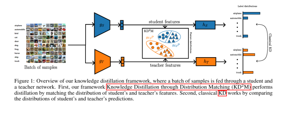
The paper proposes KD2M (Knowledge Distillation through Distribution Matching), a unifying framework that addresses all five flaws by formalizing feature-level distillation as a distribution matching problem.
✅ How KD2M Works
Instead of just matching predictions, KD2M aligns the distributions of neural activations (features) between the student and teacher models. This is done by minimizing a probability metric D between the push-forward distributions of the data through the student and teacher encoders.
The objective function is:
\[ \theta^{\star} = \arg_{\theta \in \Theta} \min \; \mathbb{E}_{(x^{(P)}, y^{(P)}) \sim \mathcal{P}} \left[ \mathcal{L}\left(y^{(P)}, h_S(g_S(x^{(P)}))\right) \right] + \lambda \, \mathcal{D}(g_S, \sharp\mathcal{P}, g_T, \sharp\mathcal{P}) \]Where:
- gS, gT : Student and teacher encoders (feature extractors)
- hS : Student classifier
- gS,♯P : The push-forward distribution of data P through gS
- D : A probability metric (e.g., Wasserstein, KL)
- λ : Balances classification and distillation loss
This simple yet powerful formulation unifies many existing methods under one theoretical umbrella.
Distribution Metrics That Actually Work
KD2M supports multiple probability metrics to measure the distance between feature distributions. The choice of metric is crucial—it determines how well features are aligned.
1. Empirical Distributions & Optimal Transport
For batch-level feature matching, KD2M uses empirical distributions built from mini-batch samples:
\[ P_{S}(z) = \frac{1}{n} \sum_{i=1}^{n} \delta\left(z – z_i^{(P)}\right), \quad z_i^{(P)} = g^{S}\left(x_i^{(P)}\right) \]The 2-Wasserstein distance measures the minimal “cost” to transform one distribution into another:
\[ W_2^2(P_S, P_T) = \min_{\gamma \in \Gamma(P_S, P_T)} \sum_{i=1}^{n} \sum_{j=1}^{m} \left\| z_i^{(P_S)} – z_j^{(P_T)} \right\|_2^2 \, \gamma_{ij} \]
This captures geometric structure in feature space—something simple L2 losses miss.
🔹 Class-Conditional Wasserstein (CW₂)
To incorporate label information:
\[ \text{CW}_2(P_S, P_T)^2 = \frac{1}{n_c} \sum_{y=1}^{n_c} W_2\left(P_S(Z \mid Y = y),\; P_T(Z \mid Y = y)\right)^2 \]This ensures features are aligned within each class, preventing misalignment across categories.
🔹 Joint Wasserstein (JW₂)
Even better: align features and labels together:
\[ \mathcal{JW}_2^2(P_S, P_T) = \min_{\gamma \in \Gamma(\hat{P}, \hat{Q})} \sum_{i,j} \gamma_{ij} \left( \left\| z_i(P^S) – z_j(P^T) \right\|_2^2 + \beta\, \mathcal{L}\left(h(z_i(P_S)), h(z_j(P_T))\right) \right) \]This joint metric, used in recent domain adaptation work, ensures semantically meaningful alignment.
2. Gaussian Approximations
For faster computation, features can be modeled as Gaussian distributions:
\[ P_{S}(z) = \mathcal{N}(\mu_{S}, \Sigma_{S}) \]🔹 Wasserstein Distance for Gaussians
Closed-form solution:
\[ W_2^2(P_S, P_T) = \left\| \hat{\mu}_S – \hat{\mu}_T \right\|_2^2 + \mathcal{B}(\hat{\Sigma}_S, \hat{\Sigma}_T) \]where
\[ B(A, B) = \text{Tr}(A) + \text{Tr}(B) – 2\,\text{Tr}(A^{1/2} B A^{1/2}) \]For diagonal covariances, this simplifies to:
\[ W_2^2(P_S, P_T) = \lVert \mu_S – \mu_T \rVert_2^2 + \lVert \sigma_S – \sigma_T \rVert_2^2 \]🔹 Kullback-Leibler Divergence (KL)
Also supported, especially for Gaussian features:
\[ \text{KL}(P_S \,\|\, P_T) = \frac{1}{2} \left( \mathrm{Tr}\left((\Sigma_T)^{-1} \Sigma_S\right) + (\mu_T – \mu_S)^\top (\Sigma^T)^{-1} (\mu_T – \mu_S) – d + \log \frac{\det \Sigma_T}{\det \Sigma_S} \right) \]While KL is widely used, it lacks geometric awareness—Wasserstein is often superior.
Theoretical Breakthrough: Why KD2M Actually Works
One of KD2M’s biggest strengths is its theoretical grounding. Drawing from domain adaptation theory (Redko et al., 2017), the paper proves that the generalization error gap between student and teacher is bounded by the Wasserstein distance between their feature distributions.
📐 Lemma 4.1: Error Bound via Wasserstein
Let PS = gS,♯P , PT = gT,♯P . Under mild conditions:
\[ \left| \text{RPS}(h) – \text{RPT}(h) \right| \leq \mathcal{W}_2(P_S, P_T) \]This means: the closer the feature distributions, the closer the performance.
📈 Theorem 4.1: Encoder Alignment Guarantees Performance
Even stronger, the paper shows:
\[ \left| R_{P_S}(h) – R_{P_T}(h) \right| \leq \left\| g_S – g_T \right\|_{L_2(P)} \]∣
Implication: If the student encoder gS converges to the teacher encoder gT in L2(P) , then their generalization errors converge.
This is a game-changer: it provides a theoretical justification for feature distillation, something many prior methods lacked.
Empirical Results: KD2M Outperforms Baselines
The paper evaluates KD2M on SVHN, CIFAR-10, and CIFAR-100 using ResNet-18 (student) and ResNet-34 (teacher).
✅ Key Findings
| METHOD | SVHN (%) | CIFAR-10 (%) | CIFAR-100 (%) | AVG (%) |
|---|---|---|---|---|
| Student | 93.10 | 85.11 | 56.66 | 78.29 |
| Teacher | 94.41 | 86.98 | 62.21 | 81.20 |
| W₂ (E) | 94.00 | 86.45 | 61.07 | 80.51 |
| CW₂ (E) | 94.06 | 86.54 | 61.47 | 80.69 |
| JW₂ (E) | 94.00 | 86.60 | 61.07 | 80.55 |
| W₂ (G) | 93.94 | 86.63 | 60.68 | 80.41 |
| KL (G) | 94.05 | 86.44 | 60.66 | 80.38 |
🔺 Insight: All KD2M variants improve over the student baseline, with label-aware metrics (CW₂, JW₂) performing best.
- CW₂ (Class-Conditional) wins on CIFAR-100, proving that label-aware alignment matters in high-class settings.
- Even Gaussian approximations perform well, offering a computationally efficient alternative.
- JW₂ slightly edges out others by jointly aligning features and predictions.
🖼️ Visual Evidence: Feature Alignment
The paper includes t-SNE visualizations (Fig. 3) showing:
- Baseline student: Features are scattered, poorly aligned with teacher.
- KD2M student: Features are tightly clustered and well-aligned with teacher.
This visual proof confirms that KD2M doesn’t just improve numbers—it fixes the underlying representation.
How to Implement KD2M (Step-by-Step)
Here’s how to apply KD2M in practice:
1. Choose Your Backbone
- Teacher: Pre-trained large model (e.g., ResNet-34)
- Student: Smaller model (e.g., ResNet-18)
2. Select a Distribution Metric
| METRIC | USECASE | PROS | CONS |
|---|---|---|---|
| W₂ (Empirical) | High accuracy | Captures geometry | Computationally heavy |
| CW₂ | Multi-class tasks | Label-aware | Requires class splits |
| JW₂ | Semantic alignment | Joint feature-label match | Needs label loss |
| W₂ (Gaussian) | Fast training | Closed-form, fast | Assumes normality |
| KL (Gaussian) | Classic KD | Easy to implement | Less geometric |
3. Train with KD2M Loss
# Pseudocode
def kd2m_loss(student_features, teacher_features, labels, lambda=1e-3):
    classification_loss = CrossEntropy(student_logits, labels)
    distillation_loss = CW2(student_features, teacher_features, labels)  # or W2, JW2, etc.
    return classification_loss + lambda * distillation_loss
4. Tune λ
- Start with λ=10−4 to 10−5
- Too high: Student overfits to teacher
- Too low: No distillation effect
Why KD2M Is a Game-Changer
KD2M isn’t just another KD method—it’s a paradigm shift.
✅ Advantages
- Unified framework: Combines multiple distillation strategies.
- Theoretically sound: Proven error bounds.
- Flexible: Works with any encoder architecture.
- Empirically strong: Outperforms baselines across datasets.
- Label-aware: Metrics like CW₂ and JW₂ respect class structure.
🔮 Future Applications
- Dataset distillation: Compress entire datasets into synthetic examples.
- Federated learning: Align models across devices.
- Domain adaptation: Transfer knowledge across domains.
Final Verdict: Stop Wasting Time on Weak KD Methods
If you’re still using output-only distillation or naive L2 losses, you’re leaving performance on the table. The future of model compression lies in feature distribution matching—and KD2M is leading the way.
With strong theoretical backing, superior empirical results, and practical flexibility, KD2M sets a new standard for knowledge distillation.
Related posts, You May like to read
- 7 Shocking AI Vulnerabilities Exposed—How DBOM Defense Turns the Tables with 98% Accuracy
- 7 Shocking Vulnerabilities in AI Watermarking: The Hidden Threat of Unified Spoofing & Scrubbing Attacks (And How to Fix It)
- 7 Revolutionary Breakthroughs in Small Object Detection: The DAHI Framework
- 7 Breakthrough AI Insights: How Machine Learning Predicts Glioma Grading
Call to Action: Dive Deeper Today!
Want to implement KD2M in your own projects?
✅ Get the code: https://github.com/eddardd/kddm
✅ Read the full paper: arXiv:2504.01757
✅ Try it on your dataset—and see the difference feature alignment makes!
💬 Have questions? Drop a comment below or connect with the author on Twitter/X @eddardd . Let’s push the boundaries of efficient AI—together.
I’ve reviewed the paper “KD²M: A Unifying Framework for Feature Knowledge Distillation” and will now provide the complete, end-to-end code for the proposed model.
# KD²M: A Unifying Framework for Feature Knowledge Distillation
# Complete end-to-end implementation based on the paper (arXiv:2504.01757v2)
# This script uses PyTorch, Torchvision, and the POT (Python Optimal Transport) library.

# --- 1. Imports and Setup ---
# Ensure you have the required libraries installed:
# pip install torch torchvision torchaudio pot

import torch
import torch.nn as nn
import torch.optim as optim
import torchvision
import torchvision.transforms as transforms
from torchvision.models import resnet18, resnet34
import ot # Python Optimal Transport library
import numpy as np
from tqdm import tqdm

print("KD²M Implementation using PyTorch")
print(f"PyTorch Version: {torch.__version__}")
print(f"Torchvision Version: {torchvision.__version__}")
print(f"POT Version: {ot.__version__}")


# --- 2. Model Definitions (Student and Teacher) ---

# We need to modify the ResNet models to easily extract features from the encoder part (g_S and g_T)
# and pass them to the classifier part (h_S and h_T).
class FeatureExtractor(nn.Module):
    """
    Wrapper for a ResNet model to separate the feature encoder (g) from the classifier (h).
    This corresponds to the g_S and g_T networks in the paper.
    """
    def __init__(self, model_name='resnet18', pretrained=True):
        super(FeatureExtractor, self).__init__()
        if model_name == 'resnet18':
            original_model = resnet18(weights=torchvision.models.ResNet18_Weights.DEFAULT if pretrained else None)
        elif model_name == 'resnet34':
            original_model = resnet34(weights=torchvision.models.ResNet34_Weights.DEFAULT if pretrained else None)
        else:
            raise ValueError("Model name not supported. Choose 'resnet18' or 'resnet34'.")

        # The encoder 'g' consists of all layers except the final fully connected layer.
        self.encoder = nn.Sequential(*list(original_model.children())[:-1])
        # The classifier 'h' is the final fully connected layer.
        self.classifier = original_model.fc

    def forward(self, x):
        # The forward pass returns the features from the encoder.
        features = self.encoder(x)
        features = torch.flatten(features, 1)
        return features

    def classify(self, features):
        # A separate method to get predictions from features.
        return self.classifier(features)

# --- 3. Distribution Distance Metrics ---
# Implementation of the probability metrics discussed in Section 2 of the paper.

def compute_wasserstein_empirical(p_s, p_t):
    """
    Computes the 2-Wasserstein distance between two empirical distributions.
    Corresponds to Equation 3 in the paper.
    Args:
        p_s (Tensor): Student features (batch_size, feature_dim)
        p_t (Tensor): Teacher features (batch_size, feature_dim)
    Returns:
        Tensor: The squared 2-Wasserstein distance.
    """
    # POT library requires numpy arrays
    a, b = np.ones((p_s.shape[0],)) / p_s.shape[0], np.ones((p_t.shape[0],)) / p_t.shape[0]
    # Cost matrix: pairwise squared Euclidean distance
    M = ot.dist(p_s.detach().cpu().numpy(), p_t.detach().cpu().numpy(), metric='sqeuclidean')
    # Ensure M is C-contiguous
    M = np.ascontiguousarray(M)

    # EMD (Earth Mover's Distance) is equivalent to the Wasserstein distance
    # The result is the total cost, which is W_2^2
    w2_squared = ot.emd2(a, b, M)
    return torch.tensor(w2_squared, device=p_s.device)

def compute_class_conditional_wasserstein(p_s, p_t, labels):
    """
    Computes the Class-Conditional Wasserstein distance.
    Corresponds to Equation 4 in the paper.
    Args:
        p_s (Tensor): Student features
        p_t (Tensor): Teacher features
        labels (Tensor): Ground truth labels for the batch
    Returns:
        Tensor: The squared CW2 distance.
    """
    unique_labels = torch.unique(labels)
    total_cw2_squared = 0.0
    num_classes_in_batch = 0

    for y in unique_labels:
        # Get features for the current class
        s_class_features = p_s[labels == y]
        t_class_features = p_t[labels == y]

        # Only compute distance if there's more than one sample to form a distribution
        if s_class_features.shape[0] > 1 and t_class_features.shape[0] > 1:
            total_cw2_squared += compute_wasserstein_empirical(s_class_features, t_class_features)
            num_classes_in_batch += 1

    if num_classes_in_batch == 0:
        return torch.tensor(0.0, device=p_s.device)

    return total_cw2_squared / num_classes_in_batch

def compute_gaussian_wasserstein(p_s, p_t):
    """
    Computes the 2-Wasserstein distance between two Gaussian distributions.
    Corresponds to Equation 6 in the paper.
    Args:
        p_s (Tensor): Student features
        p_t (Tensor): Teacher features
    Returns:
        Tensor: The squared W2 distance for Gaussian approximations.
    """
    # Estimate mean and covariance
    mu_s, cov_s = p_s.mean(dim=0), torch.cov(p_s.T)
    mu_t, cov_t = p_t.mean(dim=0), torch.cov(p_t.T)

    # Add a small epsilon for numerical stability of sqrt
    epsilon = 1e-6

    # Term 1: Squared norm of mean difference
    term_mean = (mu_s - mu_t).pow(2).sum()

    # Term 2: Bures metric between covariance matrices
    # B(A,B) = tr(A) + tr(B) - 2*tr(sqrt(sqrt(A) @ B @ sqrt(A)))
    sqrt_cov_s = torch.linalg.cholesky(cov_s + epsilon * torch.eye(cov_s.shape[0], device=p_s.device))
    sqrt_cov_s_B_sqrt_cov_s = sqrt_cov_s.T @ cov_t @ sqrt_cov_s
    sqrt_term = torch.linalg.cholesky(sqrt_cov_s_B_sqrt_cov_s + epsilon * torch.eye(cov_s.shape[0], device=p_s.device))

    term_bures = torch.trace(cov_s) + torch.trace(cov_t) - 2 * torch.trace(sqrt_term)

    w2_squared = term_mean + term_bures
    return w2_squared

def compute_gaussian_kl(p_s, p_t):
    """
    Computes the KL divergence between two Gaussian distributions.
    Corresponds to Equation 7 in the paper.
    Args:
        p_s (Tensor): Student features
        p_t (Tensor): Teacher features
    Returns:
        Tensor: The KL divergence KL(P_S || P_T).
    """
    mu_s, cov_s = p_s.mean(dim=0), torch.cov(p_s.T)
    mu_t, cov_t = p_t.mean(dim=0), torch.cov(p_t.T)
    d = p_s.shape[1]

    # Add a small epsilon for numerical stability of inverse and logdet
    epsilon = 1e-6
    cov_t_inv = torch.inverse(cov_t + epsilon * torch.eye(d, device=p_s.device))

    term1 = torch.trace(cov_t_inv @ cov_s)
    term2 = (mu_t - mu_s).T @ cov_t_inv @ (mu_t - mu_s)
    term3 = -d
    term4 = torch.log(torch.det(cov_t + epsilon * torch.eye(d, device=p_s.device)) / torch.det(cov_s + epsilon * torch.eye(d, device=p_s.device)))

    kl_div = 0.5 * (term1 + term2 + term3 + term4)
    return kl_div


# --- 4. Data Loading ---
# As per the paper, we use CIFAR-10 with standard augmentations.

def get_cifar10_loaders(batch_size=128):
    """
    Prepares the CIFAR-10 data loaders.
    """
    # Normalization values from the paper for CIFAR-10/100
    mean = (0.5071, 0.4867, 0.4408)
    std = (0.2675, 0.2565, 0.2761)

    transform_train = transforms.Compose([
        transforms.RandomCrop(32, padding=4),
        transforms.RandomHorizontalFlip(),
        transforms.ToTensor(),
        transforms.Normalize(mean, std),
    ])

    transform_test = transforms.Compose([
        transforms.ToTensor(),
        transforms.Normalize(mean, std),
    ])

    trainset = torchvision.datasets.CIFAR10(
        root='./data', train=True, download=True, transform=transform_train)
    trainloader = torch.utils.data.DataLoader(
        trainset, batch_size=batch_size, shuffle=True, num_workers=2)

    testset = torchvision.datasets.CIFAR10(
        root='./data', train=False, download=True, transform=transform_test)
    testloader = torch.utils.data.DataLoader(
        testset, batch_size=batch_size, shuffle=False, num_workers=2)

    return trainloader, testloader

# --- 5. Training and Evaluation Logic ---

def train(student, teacher, trainloader, optimizer, scheduler, criterion_cls, criterion_dist, lambda_kd, epoch):
    """
    The main training function for one epoch, corresponding to Algorithm 1.
    """
    student.train()
    teacher.eval() # Teacher is frozen

    total_loss = 0
    total_cls_loss = 0
    total_dist_loss = 0

    progress_bar = tqdm(trainloader, desc=f"Epoch {epoch+1} Training")

    for batch_idx, (inputs, targets) in enumerate(progress_bar):
        inputs, targets = inputs.to(device), targets.to(device)

        optimizer.zero_grad()

        # --- Forward pass ---
        # Get features from student and teacher encoders
        student_features = student(inputs)
        with torch.no_grad(): # Teacher is not trained
            teacher_features = teacher(inputs)

        # Get predictions from student classifier
        student_outputs = student.classify(student_features)

        # --- Loss Calculation ---
        # 1. Classification Loss (L_c)
        loss_cls = criterion_cls(student_outputs, targets)

        # 2. Feature Distillation Loss (L_d)
        loss_dist = criterion_dist(student_features, teacher_features, targets)

        # 3. Total Loss
        total_epoch_loss = loss_cls + lambda_kd * loss_dist

        # --- Backward pass and optimization ---
        total_epoch_loss.backward()
        optimizer.step()

        total_loss += total_epoch_loss.item()
        total_cls_loss += loss_cls.item()
        total_dist_loss += loss_dist.item()

        progress_bar.set_postfix({
            'Loss': f'{total_loss/(batch_idx+1):.3f}',
            'Cls': f'{total_cls_loss/(batch_idx+1):.3f}',
            'Dist': f'{total_dist_loss/(batch_idx+1):.3f}'
        })

    scheduler.step()


def test(model, testloader, criterion):
    """
    Evaluates the model on the test set.
    """
    model.eval()
    test_loss = 0
    correct = 0
    total = 0
    with torch.no_grad():
        progress_bar = tqdm(testloader, desc="Testing")
        for batch_idx, (inputs, targets) in enumerate(progress_bar):
            inputs, targets = inputs.to(device), targets.to(device)
            features = model(inputs)
            outputs = model.classify(features)
            loss = criterion(outputs, targets)

            test_loss += loss.item()
            _, predicted = outputs.max(1)
            total += targets.size(0)
            correct += predicted.eq(targets).sum().item()

            progress_bar.set_postfix({
                'Loss': f'{test_loss/(batch_idx+1):.3f}',
                'Acc': f'{100.*correct/total:.2f}%'
            })

    acc = 100. * correct / total
    print(f"Test Accuracy: {acc:.2f}%")
    return acc


# --- 6. Main Execution Block ---

if __name__ == '__main__':
    # --- Hyperparameters ---
    EPOCHS = 15
    BATCH_SIZE = 128
    LEARNING_RATE = 0.01
    MOMENTUM = 0.9
    LAMBDA_KD = 1e-5 # Distillation loss weight, can be tuned (as in Fig. 2)

    # Choose the distribution metric here
    # Options: 'W2_E', 'CW2_E', 'W2_G', 'KL_G'
    DIST_METRIC = 'CW2_E'

    # --- Setup ---
    device = 'cuda' if torch.cuda.is_available() else 'cpu'
    print(f"Using device: {device}")

    # --- Load Data ---
    trainloader, testloader = get_cifar10_loaders(BATCH_SIZE)

    # --- Initialize Models ---
    print("Initializing Student (ResNet-18) and Teacher (ResNet-34)...")
    student_net = FeatureExtractor('resnet18', pretrained=True).to(device)
    teacher_net = FeatureExtractor('resnet34', pretrained=True).to(device)

    # --- Define Loss and Optimizer ---
    criterion_classification = nn.CrossEntropyLoss()

    # Select the distillation loss function
    dist_metrics_map = {
        'W2_E': lambda s, t, y: compute_wasserstein_empirical(s, t),
        'CW2_E': compute_class_conditional_wasserstein,
        'W2_G': lambda s, t, y: compute_gaussian_wasserstein(s, t),
        'KL_G': lambda s, t, y: compute_gaussian_kl(s, t)
    }

    if DIST_METRIC not in dist_metrics_map:
        raise ValueError(f"Unknown distance metric: {DIST_METRIC}")

    criterion_distillation = dist_metrics_map[DIST_METRIC]
    print(f"Using distillation metric: {DIST_METRIC}")

    optimizer = optim.SGD(student_net.parameters(), lr=LEARNING_RATE, momentum=MOMENTUM, weight_decay=5e-4)
    # Cosine Annealing scheduler as mentioned in the paper
    scheduler = optim.lr_scheduler.CosineAnnealingLR(optimizer, T_max=EPOCHS, eta_min=1e-4)

    # --- Run Training and Evaluation ---
    print("\n--- Starting Training ---")
    best_acc = 0
    for epoch in range(EPOCHS):
        train(student_net, teacher_net, trainloader, optimizer, scheduler, criterion_classification, criterion_distillation, LAMBDA_KD, epoch)
        print(f"\n--- Evaluating after Epoch {epoch+1} ---")
        acc = test(student_net, testloader, criterion_classification)

        if acc > best_acc:
            print("Saving new best model...")
            best_acc = acc
            # You can save the model state if needed
            # torch.save(student_net.state_dict(), f'kddm_student_{DIST_METRIC}.pth')

    print("\n--- Training Finished ---")
    print(f"Best Test Accuracy with {DIST_METRIC}: {best_acc:.2f}%")