A Knowledge Distillation-Based Approach to Enhance Transparency of Classifier Models

Artificial Intelligence (AI) has revolutionized healthcare, particularly in medical image analysis. However, the “black-box” nature of deep learning models remains a significant barrier to their adoption in clinical settings. Clinicians demand not only accuracy but also transparency and interpretability—they need to understand why an AI system makes a particular diagnosis.

In response to this challenge, researchers Yuchen Jiang, Xinyuan Zhao, Yihang Wu, and Ahmad Chaddad from the Artificial Intelligence for Personalised Medicine Lab at Guilin University of Electronic Technology have proposed a novel solution: a Knowledge Distillation-Based Approach to Enhance Transparency of Classifier Models.

This groundbreaking research, detailed in their paper A Knowledge Distillation-Based Approach to Enhance Transparency of Classifier Models , introduces a method that simplifies complex Convolutional Neural Networks (CNNs) while preserving high accuracy and enabling intuitive visual explanations.

Let’s dive into how this Knowledge Distillation + Explainable AI (XAI) hybrid model works, why it matters for healthcare, and what it means for the future of trustworthy medical AI.

Why Transparency Matters in Medical AI

Before we explore the technical details, it’s essential to understand the why behind this research.

In medicine, a misdiagnosis can be life-threatening. When an AI model flags a brain tumor or detects early signs of Alzheimer’s, doctors must trust the result. But if the model cannot explain its reasoning, skepticism arises.

This is where Explainable AI (XAI) comes in. XAI methods like Grad-CAM and SHAP help visualize which parts of an image influenced the model’s decision. But these tools often struggle with large, complex models due to high computational costs and information overload.

Enter Knowledge Distillation (KD)—a technique that transfers knowledge from a large “teacher” model to a smaller, more efficient “student” model.

The team’s innovation lies in combining KD with layer-wise feature map visualization, creating a lightweight, accurate, and highly interpretable AI system tailored for medical diagnostics.

The KD-FMV Framework: Simplifying AI Without Sacrificing Performance

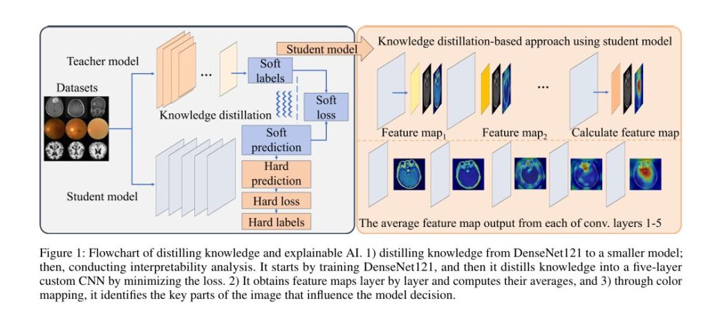
The proposed method, called Knowledge Distillation and Feature Map Visualization (KD-FMV), follows a two-step pipeline:

Train a powerful teacher model (e.g., DenseNet121) on medical image datasets.
Distill its knowledge into a smaller CNN-based student model using soft and hard loss functions.
Analyze the student model layer-by-layer using averaged feature maps to reveal decision-making processes.

This approach achieves three critical goals:

✅ High classification accuracy
✅ Reduced model complexity
✅ Enhanced interpretability

Let’s break down each component.

Step 1: Knowledge Distillation – Learning from the Expert

Knowledge Distillation works by training a smaller student model to mimic the behavior of a larger, pre-trained teacher model. The teacher has learned rich feature representations from vast data (e.g., ImageNet), and the student learns not just from labels, but from the teacher’s softened output probabilities.

The total loss function used in KD-FMV is a weighted combination of two components:

Hard Loss (Cross-Entropy with True Labels)

\[ \ell_{HL} = -\frac{1}{N} \sum_{i=1}^{N} \sum_{c=1}^{M} y_{i,c} \, \log \big( y^{S}_{i,c} \big) \]

Where:

N : number of samples
M : number of classes
y_i , c : true label (one-hot encoded)
y_S,i,c : student model’s predicted probability

Soft Loss (KL Divergence with Teacher Output)

\[ \ell_{\text{SL}}(y^{\text{true}}, y^{T}, T) = – \sum_{c=1}^{M} \; \text{softmax}(T \, y^{\text{true}}_{c}) \, \log \big( \text{softmax}(T \, y^{T}_{c}) \big) \]

Here, T is the temperature parameter, controlling the softness of the probability distribution. Higher T values make the distribution smoother, allowing the student to learn nuanced patterns.

Combined Distillation Loss

\[ L_{\text{distill}} = \alpha \cdot \ell_{HL} + (1 – \alpha) \cdot \ell_{SL} \]

Where α balances the influence of ground truth labels and teacher knowledge.

By tuning α and T , the student model achieves performance close to—or even surpassing—the teacher.

Step 2: Interpretable Analysis via Average Feature Maps

One of the biggest challenges in XAI is information overload. Deep CNNs produce dozens of feature maps per layer, making it hard to extract meaningful insights.

KD-FMV solves this by computing the average feature map across all filters in a given layer:

\[ A(i,j) = \sum_{k=1}^{N_1} F_k(i,j) \]

Where:

\[ A(i,j) \; : \; \text{average activation at spatial position } (i,j) \] \[ F_k(i,j) \; : \; \text{activation from the $k$-th filter} \] \[ N \; : \; \text{total number of filters in the layer} \]

This simple yet effective technique generates a single, clean heatmap per layer, highlighting regions that contribute most to the model’s decision.

Testing on Real Medical Datasets: Brain Tumor, Eye Disease, and Alzheimer’s

To validate their approach, the researchers tested KD-FMV on three public medical datasets:

DATASET	CLASSES	TOTAL IMAGES	TASK
Brain Tumor MRI	Glioma, Meningioma, No Tumor, Pituitary	7,023	Tumor Classification
Eye Disease (CFP)	Cataract, Diabetic Retinopathy, Glaucoma, Normal	4,217	Fundus Image Diagnosis
Alzheimer’s MRI	Mild, Moderate, Non-demented, Very Mild	~34,000	Dementia Staging

Each dataset was split into 70% training, 20% validation, 10% test (except Brain Tumor, which used an 8:2 train-test split).

The teacher model was DenseNet121 pre-trained on ImageNet. The student model was a custom 5-layer CNN with max pooling for feature retention.

Performance Results: Accuracy Meets Efficiency

Despite having far fewer layers, the student models achieved remarkable accuracy, often matching or exceeding the teacher.

Table: Classification Performance Across Datasets

MODEL	DATASET	ACCURACY	F1-SCORE	LOSS
DenseNet121 (Teacher)	Brain Tumor	0.9877	0.99	0.0621
Student (Best)	Brain Tumor	0.9748	0.98	0.0944
DenseNet121 (Teacher)	Eye Disease	0.9837	0.99	0.0490
Student (Best)	Eye Disease	0.9351	0.94	0.1956
DenseNet121 (Teacher)	Alzheimer	0.9938	0.99	0.0247
Student (Best)	Alzheimer	0.9946	0.99	0.0194

Notably, in the Alzheimer’s dataset, the student model outperformed the teacher—likely due to optimal temperature tuning during distillation.

Interpretability Analysis: Seeing How the Model Thinks

To evaluate interpretability, the team used two established XAI methods:

Grad-CAM: Highlights regions in the final convolutional layer that most influence the prediction.
SHAP (SHapley Additive exPlanations): Quantifies the contribution of each pixel to the final output.

They compared these with their proposed method (KD-FMV) using Fidelity Score, which measures how well an explanation aligns with the original model’s behavior.

Table: Fidelity Scores by Method and Dataset

DATASET	CLASS	GRAD-CAM	SHAP	OURS (KD-FMV)
Brain Tumor	Glioma	0.9639	0.9524	0.9764
	Meningioma	0.8934	0.9687	0.9161
	Pituitary	0.9322	0.9002	0.9161
	Average	0.9298	0.9404	0.9277
Eye Disease	Cataract	0.8555	0.7733	0.7852
	Diabetic Retinopathy	0.9684	0.9556	0.9080
	Glaucoma	0.8939	0.8814	0.8958
	Average	0.9059	0.8700	0.8630
Alzheimer	Mild Demented	0.9905	0.9815	0.9613
	Moderate Demented	0.9898	0.9666	0.9508
	Very Mild Demented	0.7533	0.8595	0.8274
	Average	0.9112	0.9359	0.9132

While SHAP showed slightly higher fidelity in some cases, KD-FMV delivered competitive results with significantly lower computational cost.

Time-Efficient Interpretability: Faster Insights for Faster Care

One of the most compelling advantages of KD-FMV is its computational efficiency.

Using Floating Point Operations (FLOPs) and Mean Execution Time (MET), the team showed that the student model requires less than 50% of the resources of the teacher.

Table: Computational Efficiency Comparison

MODEL	DATASET	FLOPS (x 10⁶)	MET-GRAD-CAM (S)	MET-SHAP (S)
Teacher	Brain Tumor	566.89	0.9521	67.68
Student	Brain Tumor	232.70	0.1963	15.64
Teacher	Eye Disease	566.89	0.9389	67.56
Student	Eye Disease	232.70	0.1899	15.40
Teacher	Alzheimer	566.89	0.9346	68.46
Student	Alzheimer	232.70	0.1941	15.63

💡 Key Insight: SHAP analysis dropped from ~68 seconds to ~15 seconds per image—a 78% reduction in time. This is crucial for hospitals processing thousands of scans daily.

Why This Matters: The Future of Trustworthy Medical AI

The KD-FMV framework addresses three major challenges in deploying AI in healthcare:

Model Complexity → Reduced via Knowledge Distillation
Lack of Transparency → Solved with layer-wise feature visualization
High Computational Cost → Minimized through lightweight architecture

Clinicians can now:

View heatmaps showing tumor locations in MRI scans
Track how features evolve across layers (edges → textures → objects)
Make faster, more informed decisions based on explainable outputs

Moreover, the student model’s small size makes it ideal for deployment on mobile devices, edge computing systems, or telemedicine platforms—bringing AI-powered diagnostics to remote areas.

Call to Action: Explore the Code and Join the Movement

This research isn’t just theoretical—it’s open-source and ready for real-world use.

👉 Access the full code on GitHub: https://github.com/AIPMLab/KD-FMV

You can:

Replicate the experiments
Apply KD-FMV to your own medical datasets
Contribute to the development of transparent AI in healthcare

Whether you’re a researcher, clinician, or developer, this project offers a blueprint for building accurate, efficient, and trustworthy AI models.

Conclusion: Bridging the Gap Between AI and Clinical Trust

The integration of Knowledge Distillation and Explainable AI in the KD-FMV framework represents a major step forward in medical AI. By simplifying complex models without sacrificing performance, and by enabling intuitive, layer-by-layer interpretation, this approach enhances both accuracy and trust.

As AI continues to transform medicine, transparency must be non-negotiable. Methods like KD-FMV ensure that AI doesn’t just predict—it explains, helping doctors make better decisions and ultimately improving patient outcomes.

Let’s move beyond black-box models. Let’s build AI that doctors can understand, trust, and use—every single day.

I will provide you with the complete end-to-end Python code for the model proposed in the paper “A Knowledge Distillation-Based Approach to Enhance Transparency of Classifier Models.

import tensorflow as tf
from tensorflow.keras.layers import Conv2D, MaxPooling2D, Flatten, Dense, Input, GlobalAveragePooling2D
from tensorflow.keras.models import Model
from tensorflow.keras.applications import DenseNet121
from tensorflow.keras.losses import CategoricalCrossentropy, KLDivergence
from tensorflow.keras.optimizers import Adam
import numpy as np
import matplotlib.pyplot as plt

class KD_FMV:
    """
    Implements the Knowledge Distillation and Feature Map Visualization (KD-FMV)
    approach described in the research paper.
    """

    def __init__(self, input_shape=(224, 224, 3), num_classes=4, temperature=10, alpha=0.7):
        """
        Initializes the teacher and student models, and the distiller.

        Args:
            input_shape (tuple): The shape of the input images.
            num_classes (int): The number of classes for classification.
            temperature (int): The temperature for softening probabilities.
            alpha (float): The weight to balance hard and soft loss.
        """
        self.input_shape = input_shape
        self.num_classes = num_classes
        self.temperature = temperature
        self.alpha = alpha

        # 1. Define Teacher Model (DenseNet121)
        self.teacher_model = self._build_teacher_model()

        # 2. Define Student Model (Simplified CNN)
        self.student_model = self._build_student_model()

        # 3. Combine into a Distiller model
        self.distiller = Distiller(student=self.student_model, teacher=self.teacher_model, temperature=self.temperature, alpha=self.alpha)


    def _build_teacher_model(self):
        """
        Builds the teacher model using a pre-trained DenseNet121.
        """
        base_teacher = DenseNet121(weights='imagenet', include_top=False, input_shape=self.input_shape)
        base_teacher.trainable = False # Start with pre-trained weights frozen
        inputs = Input(shape=self.input_shape)
        x = base_teacher(inputs, training=False)
        x = GlobalAveragePooling2D()(x)
        outputs = Dense(self.num_classes, activation='softmax')(x)
        teacher_model = Model(inputs, outputs, name="teacher_model")
        print("--- Teacher Model Summary ---")
        teacher_model.summary()
        return teacher_model

    def _build_student_model(self):
        """
        Builds the 5-layer student CNN model as described in the paper.
        """
        inputs = Input(shape=self.input_shape, name="student_input")
        # Layer 1
        x = Conv2D(32, (3, 3), activation='relu', padding='same', name='conv1')(inputs)
        x = MaxPooling2D((2, 2))(x)
        # Layer 2
        x = Conv2D(64, (3, 3), activation='relu', padding='same', name='conv2')(x)
        x = MaxPooling2D((2, 2))(x)
        # Layer 3
        x = Conv2D(128, (3, 3), activation='relu', padding='same', name='conv3')(x)
        x = MaxPooling2D((2, 2))(x)
        # Layer 4
        x = Conv2D(256, (3, 3), activation='relu', padding='same', name='conv4')(x)
        x = MaxPooling2D((2, 2))(x)
        # Layer 5
        x = Conv2D(512, (3, 3), activation='relu', padding='same', name='conv5')(x)
        x = MaxPooling2D((2, 2))(x)
        # Flatten and Dense layers
        x = Flatten()(x)
        outputs = Dense(self.num_classes, name="student_output")(x) # No softmax here, as it's handled in the loss
        student_model = Model(inputs, outputs, name="student_model")
        print("\n--- Student Model Summary ---")
        student_model.summary()
        return student_model

    def compile_and_train(self, train_data, epochs=10, learning_rate=1e-4):
        """
        Compiles and trains the distiller model.

        Args:
            train_data (tf.data.Dataset): The training dataset.
            epochs (int): Number of epochs to train for.
            learning_rate (float): Learning rate for the optimizer.
        """
        self.distiller.compile(
            optimizer=Adam(learning_rate=learning_rate),
            metrics=['accuracy'],
            student_loss_fn=CategoricalCrossentropy(from_logits=True),
            distillation_loss_fn=KLDivergence(),
        )
        print("\n--- Starting Student Model Training (Knowledge Distillation) ---")
        self.distiller.fit(train_data, epochs=epochs)
        print("--- Student Model Training Complete ---")

    def visualize_feature_maps(self, image):
        """
        Visualizes the average feature map for each convolutional layer in the student model.

        Args:
            image (np.array): A single input image of shape (1, H, W, C).
        """
        print(f"\n--- Generating Feature Map Visualizations for a sample image ---")
        if image.ndim == 3:
            image = np.expand_dims(image, axis=0)
            
        if image.shape != (1,) + self.input_shape:
             raise ValueError(f"Input image must have shape (1, {self.input_shape[0]}, {self.input_shape[1]}, {self.input_shape[2]}) but got {image.shape}")


        # Names of the convolutional layers in the student model
        layer_names = [layer.name for layer in self.student_model.layers if 'conv' in layer.name]
        
        # Create a model that will return the feature maps
        feature_map_model = Model(inputs=self.student_model.inputs, outputs=[self.student_model.get_layer(name).output for name in layer_names])
        
        # Get the feature maps for the input image
        feature_maps = feature_map_model.predict(image)

        # Plot the original image and the average feature maps
        num_layers = len(layer_names)
        plt.figure(figsize=(15, 4))
        
        # Original Image
        plt.subplot(1, num_layers + 1, 1)
        plt.title('Original Image')
        plt.imshow(image[0].astype('uint8'))
        plt.axis('off')

        # Average Feature Maps
        for i, (layer_name, fmap) in enumerate(zip(layer_names, feature_maps)):
            # Calculate the average feature map across all filters
            avg_fmap = np.mean(fmap[0], axis=-1)
            
            plt.subplot(1, num_layers + 1, i + 2)
            plt.title(f'Avg FMap: {layer_name}')
            plt.imshow(avg_fmap, cmap='viridis')
            plt.axis('off')
            
        plt.tight_layout()
        plt.show()

class Distiller(Model):
    """
    The Distiller model that combines the teacher and student for training.
    """
    def __init__(self, student, teacher, temperature, alpha):
        super(Distiller, self).__init__()
        self.student = student
        self.teacher = teacher
        self.temperature = temperature
        self.alpha = alpha

    def compile(self, optimizer, metrics, student_loss_fn, distillation_loss_fn):
        super(Distiller, self).compile(optimizer=optimizer, metrics=metrics)
        self.student_loss_fn = student_loss_fn
        self.distillation_loss_fn = distillation_loss_fn

    def train_step(self, data):
        x, y = data

        # Get teacher predictions (soft labels)
        teacher_predictions = self.teacher(x, training=False)

        with tf.GradientTape() as tape:
            # Get student predictions
            student_predictions = self.student(x, training=True)

            # Calculate the two losses
            student_loss = self.student_loss_fn(y, student_predictions)
            
            distillation_loss = self.distillation_loss_fn(
                tf.nn.softmax(teacher_predictions / self.temperature, axis=1),
                tf.nn.softmax(student_predictions / self.temperature, axis=1),
            )
            
            # Combine the losses
            total_loss = self.alpha * student_loss + (1 - self.alpha) * distillation_loss

        # Compute gradients
        trainable_vars = self.student.trainable_variables
        gradients = tape.gradient(total_loss, trainable_vars)

        # Update weights
        self.optimizer.apply_gradients(zip(gradients, trainable_vars))

        # Update metrics
        self.compiled_metrics.update_state(y, tf.nn.softmax(student_predictions, axis=1))

        # Return a dict of performance
        results = {m.name: m.result() for m in self.metrics}
        results.update(
            {"student_loss": student_loss, "distillation_loss": distillation_loss, "total_loss": total_loss}
        )
        return results

    def test_step(self, data):
        x, y = data
        y_prediction = self.student(x, training=False)
        student_loss = self.student_loss_fn(y, y_prediction)
        self.compiled_metrics.update_state(y, tf.nn.softmax(y_prediction, axis=1))
        results = {m.name: m.result() for m in self.metrics}
        results.update({"student_loss": student_loss})
        return results

# --- Main Execution ---
if __name__ == '__main__':
    # --- 1. Configuration ---
    IMG_HEIGHT = 224
    IMG_WIDTH = 224
    CHANNELS = 3
    NUM_CLASSES = 4 # Example: Brain Tumor (glioma, meningioma, no tumor, pituitary)
    BATCH_SIZE = 16
    EPOCHS = 5 # Using a small number for a quick demo
    TEMPERATURE = 15
    ALPHA = 0.4

    # --- 2. Create a Dummy Dataset (replace with your actual data loading) ---
    print("--- Creating a dummy dataset for demonstration ---")
    # Generate random images and one-hot encoded labels
    num_samples = 100
    dummy_images = np.random.randint(0, 256, size=(num_samples, IMG_HEIGHT, IMG_WIDTH, CHANNELS), dtype=np.uint8)
    dummy_labels_indices = np.random.randint(0, NUM_CLASSES, size=(num_samples,))
    dummy_labels_one_hot = tf.keras.utils.to_categorical(dummy_labels_indices, num_classes=NUM_CLASSES)
    
    # Create a tf.data.Dataset
    train_dataset = tf.data.Dataset.from_tensor_slices((dummy_images, dummy_labels_one_hot))
    train_dataset = train_dataset.shuffle(buffer_size=num_samples).batch(BATCH_SIZE)
    print(f"Dataset created with {num_samples} samples.")

    # --- 3. Initialize and Train the Model ---
    kd_model = KD_FMV(
        input_shape=(IMG_HEIGHT, IMG_WIDTH, CHANNELS),
        num_classes=NUM_CLASSES,
        temperature=TEMPERATURE,
        alpha=ALPHA
    )
    
    # Train the student model using knowledge distillation
    kd_model.compile_and_train(train_dataset, epochs=EPOCHS)

    # --- 4. Visualize Feature Maps for a Sample Image ---
    # Get one batch from the dataset to use for visualization
    for images, labels in train_dataset.take(1):
        sample_image = images[0]
        kd_model.visualize_feature_maps(sample_image.numpy())
        break

Related posts, You May like to read