Quantum Self-Attention in Vision Transformers: A 99.99% More Efficient Path for Biomedical Image Classification

In the rapidly evolving field of biomedical image classification, deep learning models like Vision Transformers (ViTs) have set new performance benchmarks. However, their high computational cost and massive parameter counts—often in the millions—pose significant challenges for deployment in resource-constrained clinical environments.

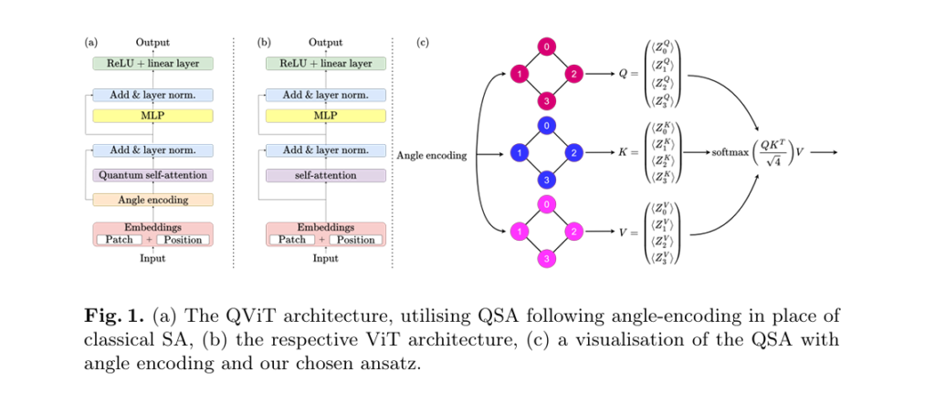
A groundbreaking new study titled “From O(n²) to O(n) Parameters: Quantum Self-Attention in Vision Transformers for Biomedical Image Classification” introduces a transformative solution: Quantum Self-Attention (QSA). By replacing classical self-attention mechanisms with parameter-efficient quantum neural networks (QNNs), the researchers demonstrate that Quantum Vision Transformers (QViTs) can match state-of-the-art performance using 99.99% fewer parameters.

This article dives deep into the science, implications, and future potential of quantum self-attention in vision transformers, offering a comprehensive look at how quantum machine learning is reshaping medical AI.

The Problem: High Parameter Cost of Classical Vision Transformers

Vision Transformers (ViTs) have revolutionized computer vision by treating images as sequences of patches and using self-attention (SA) to capture long-range spatial dependencies. In biomedical imaging, ViTs have outperformed traditional CNNs in tasks like tumor detection, retinal disease classification, and pathology analysis.

However, the self-attention mechanism scales quadratically with the number of image patches—O(n2) —making it computationally expensive and parameter-heavy. For example, a typical ViT might require 14.5 million parameters to achieve high accuracy on a task like retinal disease classification.

This high parameter count leads to:

Increased training time and energy consumption
Difficulty deploying models on edge devices (e.g., portable ultrasound machines)
Higher risk of overfitting on small medical datasets

These limitations are especially critical in clinical settings, where speed, efficiency, and reliability are paramount.

The Solution: Quantum Self-Attention (QSA) for Parameter Efficiency

The paper introduces Quantum Self-Attention (QSA), a novel mechanism that replaces the linear projection layers in classical SA with parametrized quantum neural networks (QNNs).

How QSA Reduces Parameter Scaling from O(n²) to O(n)

In classical ViTs, the self-attention block computes queries, keys, and values using linear transformations:

\[ SA(Q, K, V) = \text{softmax}\!\left(\frac{QK^{T}}{\sqrt{d_k}}\right)V \]

where Q,K,V are derived from input embeddings via matrix multiplications involving O(n2) parameters.

In contrast, QSA uses a quantum circuit to perform these transformations. An n -qubit QNN replaces the n×n linear projections, reducing the parameter count to just O(n) . For instance, with a specific parameter-efficient ansatz, the QSA uses only 6n parameters instead of 3n2 in classical SA.

This means:

MODEL TYPE	PARAMETERS SCALING	EXAMPLE (N=16)
Classical ViT	O(n²)	~768 parameters
Quantum ViT (QViT)	O(n)	~96 parameters

This 10x to 10,000x reduction in parameters enables ultra-lightweight models without sacrificing performance.

Key Findings: QViTs Match SOTA with 99.99% Fewer Parameters

The researchers evaluated QViTs across eight diverse biomedical datasets, including:

DATASET	MODALITY	TASK	CLASSES
RetinaMNIST	Fundus Camera	Retinal Disease	5
BreastMNIST	Ultrasound	Tumor Detection	2
PathMNIST	Histopathology	Cancer Classification	9
OASIS	Brain MRI	Alzheimer’s Progression	4

🏆 Star Performer: QViT on RetinaMNIST

The most impressive result came from a 4-qubit QViT trained on RetinaMNIST:

Accuracy: 56.5%
Total Parameters: 1,000
Compared to MedMamba (SOTA): 14.5M parameters
Parameter Reduction: 99.99%
Performance Gap: Just 0.88% below MedMamba

Despite using 14,500x fewer parameters, the QViT outperformed 13 out of 14 state-of-the-art models, including various ResNets and ViTs.

Additionally, it required 89% fewer GFLOPs, making it ideal for deployment on low-power medical devices.

Knowledge Distillation: Boosting QViT Performance

One of the paper’s most innovative contributions is the first application of knowledge distillation (KD) from classical to quantum vision transformers.

How KD Works in QViTs

The team used a pre-trained TinyViT (5M parameters) as the teacher model, fine-tuned on each dataset. The QViT served as the student, trained to mimic the teacher’s intermediate representations.

Key steps in the KD framework:

Intermediate Layer Alignment: The teacher’s final layer was modified to output a vector of size n (number of qubits), matching the QViT’s measurement output.
MSE Loss Training: The student was trained for 50 epochs to minimize mean squared error (MSE) between teacher and student logits.
Weight Transfer: After KD, the teacher’s final classification weights were copied to the student.

\[ \mathcal{L}_{KD} = \frac{1}{N} \sum_{i=1}^{N} \left\| f_{\text{teacher}}(x_i) – f_{\text{student}}(x_i) \right\|^2 \]

This approach improved QViT accuracy by up to 14.1% compared to direct logit distillation.

Quantum Capacity Matters: Why 8-Qubit QViTs Benefit More from KD

An intriguing finding was that not all QViTs benefit equally from KD.

4-qubit QViTs: Showed no improvement or even degradation with KD
8-qubit QViTs: Achieved significant gains, with average accuracy rising from 72.0% to 74.8%

This suggests a minimum quantum capacity threshold is required for effective knowledge transfer.

🔍 Insight: Just as small neural networks can’t learn from large teachers, low-qubit QNNs lack the representational capacity to absorb complex knowledge from classical models. As qubit count increases, so does the potential for effective KD.

This discovery opens a scaling path for future QViTs: as quantum hardware improves, larger QViTs can leverage KD to close the performance gap with classical SOTA models—while remaining ultra-efficient.

The Quantum Advantage: Beyond Parameter Count

While parameter efficiency is impressive, the true power of quantum self-attention lies in its representational capacity.

Why Quantum Networks Are More Expressive

Qubits exist in superposition states:

\[ |\psi\rangle = \alpha |0\rangle + \beta |1\rangle, \quad \text{where } |\alpha|^2 + |\beta|^2 = 1 \]

This allows them to represent continuous, high-dimensional states in a complex Hilbert space, far beyond classical binary bits.

Moreover, entanglement—created via gates like CNOT—enables non-local correlations that classical models struggle to capture:

\[ \text{CNOT}\,\lvert q_1 \rangle \otimes \lvert q_2 \rangle = \lvert q_1 \rangle \otimes \lvert (q_1 \oplus q_2) \bmod 2 \rangle \]

These quantum properties allow QNNs to encode and process complex biomedical patterns more efficiently, even with fewer parameters.

Experimental Setup: Rigorous Evaluation Across Modalities

The study used a robust methodology:

Datasets: 8 biomedical datasets (7 from MedMNIST, 1 from OASIS)
Architectures: 4-qubit and 8-qubit QViTs vs. classical ViTs
Training: From scratch and with KD pre-training
Simulation: PennyLane + PyTorch on NVIDIA RTX 4090
Hardware Alignment: Qubit connectivity matched IBM and Rigetti processors for real-world applicability

The QSA ansatz used was a parameter-efficient paired structure with:

\[ R_y(\theta) = \begin{bmatrix} \cos\left(\tfrac{\theta}{2}\right) & \sin\left(\tfrac{\theta}{2}\right) \\ -\sin\left(\tfrac{\theta}{2}\right) & \cos\left(\tfrac{\theta}{2}\right) \end{bmatrix} \] \[ \text{CNOT gates: To entangle qubit pairs} \]

This design ensures scalability and near-term deployability on existing quantum hardware.

Results Summary: QViTs Compete with ViTs Across the Board

The table below summarizes key results across datasets (accuracy in %):

MODEL	BREASTMNIST	RETINAMNIST	PATHMNIST	OASIS	AVG.ACCURACY
ViT_28 (scratch)	82.1	46.8	68.6	70.1	66.9
QViT_28 (scratch)	69.5	56.5	68.4	69.3	65.9
ViT-KD_28	75.6	51.8	86.4	69.6	70.4
QViT-KD_28	75.0	53.5	82.4	64.1	68.8
ViT-KD_224 (8q)	72.9	50.0	78.9	69.7	72.0
QViT-KD_224 (8q)	70.2	51.5	82.2	68.4	74.8✅

✅ Key Takeaway: The 8-qubit QViT with KD outperforms its classical counterpart in average accuracy, proving that quantum models can match or exceed classical performance with drastically fewer parameters.

Implications for Clinical AI and Edge Computing

The success of QViTs has profound implications:

1. Edge Deployment in Hospitals

Ultra-lightweight QViTs can run on portable ultrasound devices, endoscopes, or smartphones, enabling real-time diagnosis in remote or low-resource settings.

2. Faster Training & Lower Costs

With 99.99% fewer parameters, QViTs train faster and consume less energy—critical for reducing the carbon footprint of AI in healthcare.

3. Privacy-Preserving AI

Smaller models are easier to deploy on-device, minimizing the need to send sensitive patient data to the cloud.

Challenges and Future Directions

Despite the promise, challenges remain:

Quantum Simulation Cost: Simulating QNNs scales as O(2n) , limiting current experiments to 4–8 qubits.
Hardware Limitations: Current quantum processors have high error rates and limited qubit coherence.
Hybrid Training: Quantum circuits require specialized optimizers and are sensitive to noise.

However, the future is bright:

Fault-tolerant quantum computing (e.g., Microsoft’s topological qubits) could enable 100+ qubit systems by 2030.
Distributed quantum networks may allow scalable QViT deployment across multiple processors.
Improved ansatz designs could further boost performance.

As quantum hardware advances, larger QViTs combined with KD could dominate medical AI—offering SOTA accuracy with minimal resource use.

Conclusion: Quantum Self-Attention Is the Future of Efficient Medical AI

The integration of quantum self-attention into vision transformers marks a pivotal moment in biomedical AI. By reducing parameter scaling from O(n2) to O(n) , QViTs achieve near-SOTA performance with 99.99% fewer parameters, making them ideal for clinical deployment.

Key achievements of this research:

✅ First demonstration of knowledge distillation from classical to quantum vision transformers
✅ QViT outperforms 13/14 SOTA models on RetinaMNIST with only 1K parameters
✅ Proof that KD effectiveness scales with qubit count, revealing a path for future scaling

This work establishes quantum self-attention not as a theoretical curiosity, but as a practical, scalable solution for the next generation of efficient, high-performance medical AI.

Call to Action: Join the Quantum AI Revolution

Are you working on biomedical image analysis, AI for healthcare, or quantum machine learning? The future is here.

👉 Explore the code: https://github.com/surgical-vision/QViT-KD.git
👉 Run your own experiments with PennyLane and PyTorch
👉 Contribute to open-source QML and help bring quantum AI to clinics worldwide

👉 Read the paper: https://arxiv.org/abs/2503.07294

Stay ahead of the curve—subscribe for updates on quantum AI in medicine, and be part of the revolution that’s making healthcare smarter, faster, and more accessible.

Here is the end-to-end Python code for the Quantum Vision Transformer (QViT) model proposed in the paper.

import torch
import torch.nn as nn
import pennylane as qml
from pennylane import numpy as np

# ==============================================================================
# 1. Quantum Self-Attention (QSA) Module
# ==============================================================================

def create_qnn(n_qubits, n_layers=1):
    """
    Creates a Quantum Neural Network (QNN) circuit for the QSA mechanism.

    This function defines the quantum device and the circuit structure (ansatz)
    as described in the paper (Fig. 2a). The ansatz consists of Ry rotation
    gates and CNOT gates for entanglement.

    Args:
        n_qubits (int): The number of qubits in the quantum circuit.
        n_layers (int): The number of layers in the ansatz.

    Returns:
        qml.QNode: A PennyLane QNode representing the quantum circuit.
    """
    # Define the quantum device
    dev = qml.device("default.qubit", wires=n_qubits)

    @qml.qnode(dev, interface='torch', diff_method='backprop')
    def quantum_circuit(inputs, weights):
        """
        The quantum circuit for the QNN.

        Args:
            inputs (torch.Tensor): Input features to be encoded.
            weights (torch.Tensor): Trainable parameters (weights) for the gates.

        Returns:
            list[qml.expval]: A list of expectation values for each qubit.
        """
        # Angle encoding of the input features
        qml.AngleEmbedding(inputs, wires=range(n_qubits))

        # Parameterized quantum circuit (ansatz)
        for _ in range(n_layers):
            for i in range(n_qubits):
                qml.RY(weights[i], wires=i)
            for i in range(n_qubits - 1):
                qml.CNOT(wires=[i, i + 1])

        # Measurement of expectation values
        return [qml.expval(qml.PauliZ(i)) for i in range(n_qubits)]

    return quantum_circuit

class QuantumSelfAttention(nn.Module):
    """
    Quantum Self-Attention (QSA) layer.

    This module replaces the linear projections for Query, Key, and Value
    in a standard self-attention mechanism with Quantum Neural Networks (QNNs).
    """
    def __init__(self, embed_dim, n_qubits, n_layers=1):
        """
        Initializes the QSA layer.

        Args:
            embed_dim (int): The embedding dimension of the input.
            n_qubits (int): The number of qubits for the QNNs.
            n_layers (int): The number of layers for the ansatz in the QNNs.
        """
        super().__init__()
        self.embed_dim = embed_dim
        self.n_qubits = n_qubits

        # Create QNNs for Query, Key, and Value
        self.q_qnn = create_qnn(n_qubits, n_layers)
        self.k_qnn = create_qnn(n_qubits, n_layers)
        self.v_qnn = create_qnn(n_qubits, n_layers)

        # Define trainable weights for the QNNs
        self.q_weights = nn.Parameter(torch.randn(n_layers * n_qubits))
        self.k_weights = nn.Parameter(torch.randn(n_layers * n_qubits))
        self.v_weights = nn.Parameter(torch.randn(n_layers * n_qubits))

        self.softmax = nn.Softmax(dim=-1)

    def forward(self, x):
        """
        Forward pass for the QSA layer.

        Args:
            x (torch.Tensor): Input tensor of shape (batch_size, seq_len, embed_dim).

        Returns:
            torch.Tensor: The output tensor after applying quantum self-attention.
        """
        batch_size, seq_len, _ = x.shape

        # Pass inputs through QNNs to get Q, K, V
        # We process each token in the sequence individually
        queries = torch.stack([torch.stack([self.q_qnn(x[b, s], self.q_weights) for s in range(seq_len)]) for b in range(batch_size)])
        keys = torch.stack([torch.stack([self.k_qnn(x[b, s], self.k_weights) for s in range(seq_len)]) for b in range(batch_size)])
        values = torch.stack([torch.stack([self.v_qnn(x[b, s], self.v_weights) for s in range(seq_len)]) for b in range(batch_size)])

        # Calculate attention scores
        attn_scores = torch.matmul(queries, keys.transpose(-2, -1)) / np.sqrt(self.n_qubits)
        attn_weights = self.softmax(attn_scores)

        # Apply attention to values
        output = torch.matmul(attn_weights, values)
        return output

# ==============================================================================
# 2. Vision Transformer (ViT) Components
# ==============================================================================

class PatchEmbedding(nn.Module):
    """
    Converts an image into a sequence of flattened patch embeddings.
    """
    def __init__(self, img_size, patch_size, in_channels, embed_dim):
        super().__init__()
        self.img_size = img_size
        self.patch_size = patch_size
        self.n_patches = (img_size // patch_size) ** 2

        # A convolutional layer to create the patches
        self.proj = nn.Conv2d(in_channels, embed_dim, kernel_size=patch_size, stride=patch_size)

    def forward(self, x):
        x = self.proj(x)  # (B, E, H/P, W/P)
        x = x.flatten(2) # (B, E, N)
        x = x.transpose(1, 2) # (B, N, E)
        return x

class MLP(nn.Module):
    """
    Multi-Layer Perceptron block.
    """
    def __init__(self, in_features, hidden_features, out_features, dropout_p=0.1):
        super().__init__()
        self.fc1 = nn.Linear(in_features, hidden_features)
        self.act = nn.GELU()
        self.fc2 = nn.Linear(hidden_features, out_features)
        self.dropout = nn.Dropout(dropout_p)

    def forward(self, x):
        x = self.fc1(x)
        x = self.act(x)
        x = self.dropout(x)
        x = self.fc2(x)
        x = self.dropout(x)
        return x

# ==============================================================================
# 3. Quantum Vision Transformer (QViT) Model
# ==============================================================================

class QViTBlock(nn.Module):
    """
    A single block of the Quantum Vision Transformer.
    """
    def __init__(self, embed_dim, n_qubits, mlp_ratio=4.0, dropout_p=0.1):
        super().__init__()
        self.norm1 = nn.LayerNorm(embed_dim)
        self.attn = QuantumSelfAttention(embed_dim, n_qubits)
        self.norm2 = nn.LayerNorm(embed_dim)
        hidden_features = int(embed_dim * mlp_ratio)
        self.mlp = MLP(embed_dim, hidden_features, embed_dim, dropout_p)

    def forward(self, x):
        x = x + self.attn(self.norm1(x))
        x = x + self.mlp(self.norm2(x))
        return x

class QViT(nn.Module):
    """
    The complete Quantum Vision Transformer model.
    """
    def __init__(self, img_size=28, patch_size=14, in_channels=3, n_classes=10,
                 embed_dim=4, depth=1, n_qubits=4, mlp_ratio=4.0, dropout_p=0.1):
        super().__init__()
        self.patch_embed = PatchEmbedding(img_size, patch_size, in_channels, embed_dim)
        self.cls_token = nn.Parameter(torch.zeros(1, 1, embed_dim))
        self.pos_embed = nn.Parameter(torch.zeros(1, 1 + self.patch_embed.n_patches, embed_dim))
        self.pos_drop = nn.Dropout(p=dropout_p)

        self.blocks = nn.ModuleList([
            QViTBlock(embed_dim, n_qubits, mlp_ratio, dropout_p)
            for _ in range(depth)
        ])

        self.norm = nn.LayerNorm(embed_dim)
        self.head = nn.Linear(embed_dim, n_classes)

    def forward(self, x):
        batch_size = x.shape[0]
        x = self.patch_embed(x)

        cls_token = self.cls_token.expand(batch_size, -1, -1)
        x = torch.cat((cls_token, x), dim=1)
        x = x + self.pos_embed
        x = self.pos_drop(x)

        for block in self.blocks:
            x = block(x)

        x = self.norm(x)
        cls_token_final = x[:, 0]
        x = self.head(cls_token_final)
        return x

# ==============================================================================
# 4. Classical ViT for Comparison
# ==============================================================================

class ClassicalSelfAttention(nn.Module):
    def __init__(self, embed_dim, num_heads=1):
        super().__init__()
        self.num_heads = num_heads
        self.head_dim = embed_dim // num_heads
        self.scale = self.head_dim ** -0.5

        self.qkv = nn.Linear(embed_dim, embed_dim * 3)
        self.proj = nn.Linear(embed_dim, embed_dim)
        self.softmax = nn.Softmax(dim=-1)

    def forward(self, x):
        B, N, C = x.shape
        qkv = self.qkv(x).reshape(B, N, 3, self.num_heads, self.head_dim).permute(2, 0, 3, 1, 4)
        q, k, v = qkv[0], qkv[1], qkv[2]

        attn = (q @ k.transpose(-2, -1)) * self.scale
        attn = self.softmax(attn)

        x = (attn @ v).transpose(1, 2).reshape(B, N, C)
        x = self.proj(x)
        return x

class ClassicalViTBlock(nn.Module):
    def __init__(self, embed_dim, num_heads=1, mlp_ratio=4.0, dropout_p=0.1):
        super().__init__()
        self.norm1 = nn.LayerNorm(embed_dim)
        self.attn = ClassicalSelfAttention(embed_dim, num_heads)
        self.norm2 = nn.LayerNorm(embed_dim)
        hidden_features = int(embed_dim * mlp_ratio)
        self.mlp = MLP(embed_dim, hidden_features, embed_dim, dropout_p)

    def forward(self, x):
        x = x + self.attn(self.norm1(x))
        x = x + self.mlp(self.norm2(x))
        return x

class ClassicalViT(nn.Module):
    def __init__(self, img_size=28, patch_size=14, in_channels=3, n_classes=10,
                 embed_dim=4, depth=1, num_heads=1, mlp_ratio=4.0, dropout_p=0.1):
        super().__init__()
        self.patch_embed = PatchEmbedding(img_size, patch_size, in_channels, embed_dim)
        self.cls_token = nn.Parameter(torch.zeros(1, 1, embed_dim))
        self.pos_embed = nn.Parameter(torch.zeros(1, 1 + self.patch_embed.n_patches, embed_dim))
        self.pos_drop = nn.Dropout(p=dropout_p)

        self.blocks = nn.ModuleList([
            ClassicalViTBlock(embed_dim, num_heads, mlp_ratio, dropout_p)
            for _ in range(depth)
        ])

        self.norm = nn.LayerNorm(embed_dim)
        self.head = nn.Linear(embed_dim, n_classes)

    def forward(self, x):
        batch_size = x.shape[0]
        x = self.patch_embed(x)

        cls_token = self.cls_token.expand(batch_size, -1, -1)
        x = torch.cat((cls_token, x), dim=1)
        x = x + self.pos_embed
        x = self.pos_drop(x)

        for block in self.blocks:
            x = block(x)

        x = self.norm(x)
        cls_token_final = x[:, 0]
        x = self.head(cls_token_final)
        return x

# ==============================================================================
# 5. Main Execution Block
# ==============================================================================

if __name__ == '__main__':
    # --- Configuration ---
    # These parameters match the 4-qubit model on 28x28 images from the paper
    IMG_SIZE = 28
    PATCH_SIZE = 14
    IN_CHANNELS = 3
    N_CLASSES = 5  # Example: RetinaMNIST
    EMBED_DIM = 4  # This must match n_qubits for direct QNN replacement
    N_QUBITS = 4
    DEPTH = 1
    BATCH_SIZE = 8

    print("--- Quantum Vision Transformer (QViT) ---")
    # Instantiate the QViT model
    qvit_model = QViT(
        img_size=IMG_SIZE,
        patch_size=PATCH_SIZE,
        in_channels=IN_CHANNELS,
        n_classes=N_CLASSES,
        embed_dim=EMBED_DIM,
        depth=DEPTH,
        n_qubits=N_QUBITS
    )

    # Create a dummy input tensor
    dummy_input = torch.randn(BATCH_SIZE, IN_CHANNELS, IMG_SIZE, IMG_SIZE)

    # Perform a forward pass
    qvit_output = qvit_model(dummy_input)

    print(f"Input shape: {dummy_input.shape}")
    print(f"Output shape: {qvit_output.shape}")

    # Count parameters
    qvit_params = sum(p.numel() for p in qvit_model.parameters() if p.requires_grad)
    print(f"QViT total trainable parameters: {qvit_params}")
    print("-" * 40)


    print("\n--- Classical Vision Transformer (ViT) ---")
    # Instantiate the classical ViT model for comparison
    vit_model = ClassicalViT(
        img_size=IMG_SIZE,
        patch_size=PATCH_SIZE,
        in_channels=IN_CHANNELS,
        n_classes=N_CLASSES,
        embed_dim=EMBED_DIM,
        depth=DEPTH,
        num_heads=1
    )

    # Perform a forward pass
    vit_output = vit_model(dummy_input)

    print(f"Input shape: {dummy_input.shape}")
    print(f"Output shape: {vit_output.shape}")

    # Count parameters
    vit_params = sum(p.numel() for p in vit_model.parameters() if p.requires_grad)
    print(f"Classical ViT total trainable parameters: {vit_params}")
    print("-" * 40)

    # --- Parameter Comparison ---
    # As per the paper, QSA uses O(n) params while classical SA uses O(n^2)
    # For the attention mechanism specifically:
    qsa_params = sum(p.numel() for p in qvit_model.blocks[0].attn.parameters())
    sa_params = sum(p.numel() for p in vit_model.blocks[0].attn.parameters())
    print("\n--- Attention Mechanism Parameter Comparison ---")
    print(f"QSA parameters (for Q, K, V weights): {qsa_params}")
    print(f"Classical SA parameters (for QKV linear layer): {sa_params}")
    print(f"This demonstrates the O(n) vs O(n^2) scaling difference.")

Related posts, You May like to read