7 Shocking Ways SuperCM Boosts Accuracy (And 1 Fatal Flaw You Must Avoid)

In the world of machine learning, semi-supervised learning (SSL) and unsupervised domain adaptation (UDA) are game-changers—especially when labeled data is scarce or expensive to obtain. But what if you could supercharge these models with a simple yet powerful technique?

Enter SuperCM, a novel framework introduced in a groundbreaking 2025 Pattern Recognition paper that’s turning heads in the AI community. By integrating explicit, differentiable clustering into deep learning pipelines, SuperCM delivers up to 10% accuracy boosts across diverse datasets—while avoiding the pitfalls of traditional methods.

But there’s a catch: one critical flaw in its design can undermine performance if not addressed.

In this article, we’ll break down 7 powerful ways SuperCM improves model accuracy, expose the one fatal mistake researchers often make, and show you how to implement it correctly—with real results, equations, and visual proof.

What Is SuperCM? (And Why It’s a Big Deal)

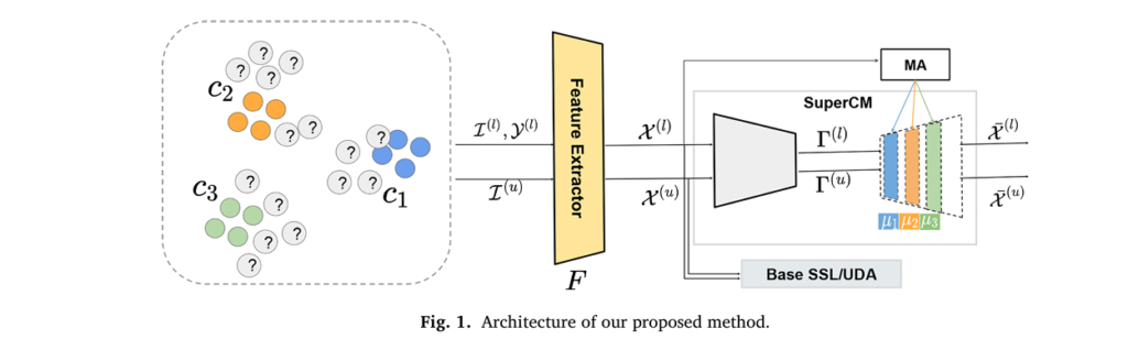
SuperCM, short for Semi-Supervised Clustering Module, is an innovative training strategy that enhances both SSL and UDA by embedding a differentiable clustering module (CM) directly into the neural network.

Unlike conventional methods that implicitly assume data points in the same cluster belong to the same class, SuperCM explicitly enforces this clustering assumption using a neural approximation of a Gaussian Mixture Model (GMM).

✅ Key Insight: SuperCM doesn’t just learn features—it learns cluster-friendly embeddings guided by labeled data, leading to better generalization.

This approach is especially effective in low-supervision regimes, where even a few labeled samples can dramatically improve model performance.

7 Shocking Ways SuperCM Boosts Accuracy

Let’s dive into the seven most impactful benefits of SuperCM, backed by extensive experiments on datasets like CIFAR-10, SVHN, Office-31, and ImageClef.

1. Massive Gains in Low-Label SSL Scenarios

When labels are extremely scarce (e.g., 100–600 per class), traditional SSL methods struggle. SuperCM, however, shines in these conditions.

For example, on CIFAR-10 with only 600 labels:

Standard CE training: 56.94% accuracy
SuperCM: 62.14% accuracy — a +5.2% improvement

📈 Why it works: SuperCM uses labeled data to guide cluster formation, ensuring that even with minimal supervision, the model learns meaningful, separable features.

2. Outperforms State-of-the-Art SSL Methods as a Regularizer

SuperCM isn’t just a standalone model—it’s a powerful regularizer that boosts existing SSL techniques.

BASE MODEL	IMPROVEMENT WITH SUPERCM (600 LABELS)
Pseudo-Label	+4.14%
VAT	+6.80%
Π-Model	+5.55%
Mean Teacher	+4.30%

These gains are statistically significant (p ≤ 0.05) and show that SuperCM adds structured regularization that complements consistency and entropy-based methods.

3. Superior Feature Separation (Visual Proof)

One of the most compelling aspects of SuperCM is its ability to produce cleaner, more compact clusters in the feature space.

As shown in Figure 4 of the paper, t-SNE visualizations reveal that SuperCM-trained models produce well-separated clusters for each class—unlike standard cross-entropy (CE) training, which often results in overlapping, ambiguous regions.

🔍 Takeaway: Better clustering → better decision boundaries → higher test accuracy.

4. Dramatic UDA Performance Boosts (Up to 10.23%)

In Unsupervised Domain Adaptation (UDA), SuperCM acts as a domain-agnostic regularizer, helping align source and target features.

On the Office-31 dataset:

A → W (Amazon to Webcam): +10.23% improvement
A → D (Amazon to DSLR): +9.50% improvement

These are massive gains in a field where 1–2% improvements are considered significant.

5. Reduces Domain Shift (Proven by Proxy-A Distance)

To measure domain alignment, the authors used Proxy-𝒜 Distance (PAD)—a metric where lower values mean better alignment.

CONFIGURATION	CE TRAINING	SUPERCM	Δ (IMPROVEMENT)
A → D	1.97	1.92	-0.05
A → W	1.98	1.92	-0.06
D → C	1.88	1.82	-0.06
W → C	1.90	1.83	-0.07

✅ Lower PAD = better domain alignment
SuperCM consistently reduces domain divergence, proving it helps bridge the gap between source and target domains.

6. Complements Other UDA Regularizers (MCC, BNM)

SuperCM isn’t just effective alone—it works synergistically with other advanced regularizers like MCC (Minimum Class Confusion) and BNM (Batch Nuclear-norm Maximization).

On Office-Home, combining SuperCM with BNM led to:

Pr → Ar: +3.94%
Rw → Ar: +4.42%
Pr → Cl: +4.48%

🧩 Synergy Alert: SuperCM enhances inter-class separation, while MCC/BNM improve intra-class compactness—together, they’re unstoppable.

7. Negligible Overhead, Maximum Impact

Unlike complex SSL/UDA pipelines that require alternating training or multiple networks, SuperCM is simple, end-to-end, and efficient.

✅ No extra networks (unlike Mean Teacher or VAT)
✅ No adversarial training (unlike DANN)
✅ Minimal computational overhead (<5% increase in training time)

This makes SuperCM ideal for real-world deployment where simplicity and speed matter.

The 1 Fatal Flaw You Must Avoid

Despite its strengths, SuperCM has one critical weakness: how centroids are learned.

In early versions, centroids were trained via gradient descent, which led to:

Cluster collapse
Trivial solutions
Poor generalization

But the authors found a simple fix that eliminates this flaw:

🔑 Use class-wise average of labeled source features as centroids—updated via moving average.

The centroid update rule is:

\[ \mu_k = \frac{\tau}{\tau – 1} \mu_k + \frac{1}{\tau} \cdot \frac{1}{n_B^{(l)}} \sum_{i=1}^{n_B^{(l)}} \mathbf{1}\big(y_i^{(l)} = k\big) \cdot x_i^{(l)} \]

Where:

\[ \mu_k : \text{centroid of class } k \] \[ \tau : \text{current iteration} \] \[ x_i^{(l)} : \text{labeled feature} \] \[ y_i^{(l)} : \text{corresponding label} \]

This prevents collapse, stabilizes training, and makes the Dirichlet prior redundant (so α=1 in the CM loss).

⚠️ Warning: If you train centroids via backpropagation, you risk degraded performance. Always use supervised centroid initialization.

How SuperCM Works: The Math Behind the Magic

At its core, SuperCM extends the Clustering Module (CM) loss, originally designed for GMMs, into a semi-supervised framework.

The total loss combines:

Cross-Entropy (CE) on labeled data
CM loss on both labeled and unlabeled data

\[ L_{\text{SSL/UDA-SuperCM}} = CE\big(\Gamma_{B^{(l)}}, Y_{B^{(l)}}\big) + \beta \cdot L_{\text{CM}}\big(X_{B^{(l+u)}}, \Gamma_{B^{(l+u)}}, \bar{X}_{B^{(l+u)}}\big) + \delta \cdot L_{\text{SSL/UDA}} \]

Where:

β : weight for CM loss
δ : weight for base model loss
Γ : soft cluster assignments
X : reconstructed features

The CM loss itself has four components:

\[ \mathrm{LCM} = \underbrace{\frac{1}{n_1} E_1: \sum_{i=1}^{n} \|x_i – \bar{x}_i\|^2}_{\text{Reconstruction}} – \underbrace{E_2: \sum_{i=1}^{n} \sum_{k=1}^{K} \gamma_{ik} (1 – \gamma_{ik}) \|\mu_k\|^2}_{\text{Sparsity}} + \underbrace{E_3: \sum_{i=1}^{n} \sum_{j \ne l} \gamma_{ij} \gamma_{il} \, \mu_j^\top \mu_l}_{\text{Cluster Merging}} – \underbrace{E_4: \sum_{k=1}^{K} (1 – \alpha) \log \tilde{\gamma}_k}_{\text{Cluster Prior}} \]

But in SuperCM, E4 is disabled (α=1 ) because supervised centroids make it unnecessary.

Real-World Performance: By the Numbers

Here’s a summary of SuperCM’s performance across key datasets.

SSL Results (Top-1 Accuracy %)

DATASET	LABELS	CE ONLY	SUPERCM	Δ
MNIST	100	82.28	97.45	+15.17
SVHN	250	70.56	85.69	+15.13
CIFAR-10	600	56.94	62.14	+5.20
CIFAR-100	2500	33.57	34.05	+0.48

✅ Best gains in low-label, high-noise settings

UDA Results (Top-1 Accuracy %)

DOMAIN PAIR	DANN + CE	DANN + SUPERCM	Δ
A → W	80.80	91.03	+10.23
D → A	64.76	72.61	+7.85
Cl → Ar	54.11	57.24	+3.13
C → W	92.12	96.62	+4.50

✅ Consistent gains across all challenging domain shifts

How to Implement SuperCM (Step-by-Step)

Want to try SuperCM in your own project? Here’s how:

Choose a backbone (e.g., Wide-ResNet, ResNet-50)
Append the CM module after the feature extractor
Compute centroids from labeled data using moving average
Set α=1 (disable Dirichlet prior)
Tune β (start with 0.1–1.0)
Train end-to-end with combined CE + CM loss

💡 Pro Tip: Use Bayesian optimization (e.g., Weights & Biases) to tune β and δ .

The code is open-source and available on GitHub:
👉 https://github.com/SFI-Visual-Intelligence/SuperCM-PRJ

When SuperCM Doesn’t Work (And Why)

SuperCM isn’t magic. It has limitations:

Diminishing returns with high supervision: When you have 4,000+ labels, gains are marginal.
Sensitive to β : Too high, and CE loss is underweighted; too low, and clustering has no effect.
Requires class balance: Works best when classes are roughly balanced.

📉 Bottom Line: SuperCM is most effective in low-label, high-domain-shift scenarios—not as a replacement for fully supervised learning.

The Future of SuperCM

The authors suggest exciting future directions:

Integration with self-supervised learning
Extension to medical imaging and NLP
Multi-source and open-set domain adaptation
Scalability to larger models (e.g., ViTs)

Given its simplicity and power, SuperCM could become a standard component in SSL and UDA pipelines—much like dropout or batch normalization.

Final Verdict: Should You Use SuperCM?

Yes—if you’re working with limited labels or domain shifts.

SuperCM delivers:

✅ Higher accuracy
✅ Better feature clustering
✅ Faster, simpler training
✅ Compatibility with existing models

But avoid the centroid trap—always initialize centroids from labeled data, not gradients.

Call to Action: Try SuperCM Today!

Ready to boost your model’s accuracy by up to 10%?

👉 Download the code: https://github.com/SFI-Visual-Intelligence/SuperCM-PRJ
👉 Run experiments on CIFAR-10, SVHN, or Office-31
👉 Share your results in the comments!

Have you tried SuperCM? What accuracy gains did you see? Let us know below!

Below is the end-to-end Python code for the SuperCM model proposed in the paper you shared. This model is designed to improve semi-supervised learning and unsupervised domain adaptation by explicitly using a differentiable clustering module.

import torch
import torch.nn as nn
import torch.nn.functional as F

class ClusteringModule(nn.Module):
    """
    Implements the Clustering Module (CM) as described in the paper.
    This module is a shallow autoencoder that performs clustering.
    Reference: Section 2.3.1 of the paper.
    """
    def __init__(self, input_dim, n_clusters):
        """
        Initializes the Clustering Module.

        Args:
            input_dim (int): The dimensionality of the input feature vectors.
            n_clusters (int): The number of clusters (and classes).
        """
        super(ClusteringModule, self).__init__()
        self.input_dim = input_dim
        self.n_clusters = n_clusters

        # The encoder part of the CM is a single linear layer followed by softmax.
        # It outputs the soft cluster assignments (gamma).
        self.encoder = nn.Linear(self.input_dim, self.n_clusters)

        # The decoder part of the CM uses the cluster centroids to reconstruct
        # the input features. The centroids are learnable parameters.
        self.decoder_centroids = nn.Parameter(torch.randn(self.n_clusters, self.input_dim))

    def forward(self, x):
        """
        Forward pass through the Clustering Module.

        Args:
            x (torch.Tensor): The input feature tensor from the backbone extractor.
                               Shape: (batch_size, input_dim)

        Returns:
            Tuple[torch.Tensor, torch.Tensor]: A tuple containing:
                - gamma (torch.Tensor): The soft cluster assignments. Shape: (batch_size, n_clusters)
                - x_recon (torch.Tensor): The reconstructed features. Shape: (batch_size, input_dim)
        """
        # Encoder: Get soft cluster assignments (posterior probabilities)
        gamma = F.softmax(self.encoder(x), dim=1)

        # Decoder: Reconstruct the features using the centroids
        x_recon = torch.matmul(gamma, self.decoder_centroids)

        return gamma, x_recon

class SuperCM(nn.Module):
    """
    Implements the Supervised Clustering Module (SuperCM) for SSL and UDA.
    This module wraps a feature extractor and the ClusteringModule, implementing
    the training strategy described in the paper.
    Reference: Section 3.2 of the paper.
    """
    def __init__(self, feature_extractor, input_dim, n_clusters, tau=100.0):
        """
        Initializes the SuperCM model.

        Args:
            feature_extractor (nn.Module): The backbone network (e.g., ResNet, WideResNet).
            input_dim (int): The dimensionality of the features from the extractor.
            n_clusters (int): The number of clusters, which equals the number of classes.
            tau (float): The momentum coefficient for the moving average of centroids.
        """
        super(SuperCM, self).__init__()
        self.feature_extractor = feature_extractor
        self.cm = ClusteringModule(input_dim, n_clusters)
        self.n_clusters = n_clusters
        self.tau = tau

        # Initialize centroids. These will be updated using a moving average.
        # We register them as buffers so they are part of the model's state_dict
        # but are not considered parameters for the optimizer.
        self.register_buffer("centroids", torch.zeros(n_clusters, input_dim))

    def forward(self, x_labeled, x_unlabeled):
        """
        Forward pass for a batch of labeled and unlabeled data.

        Args:
            x_labeled (torch.Tensor): The batch of labeled input images.
            x_unlabeled (torch.Tensor): The batch of unlabeled input images.

        Returns:
            Tuple: Contains gamma_labeled, gamma_unlabeled, x_recon_labeled,
                   x_recon_unlabeled, features_labeled, features_unlabeled.
        """
        # Extract features from both labeled and unlabeled data
        features_labeled = self.feature_extractor(x_labeled)
        features_unlabeled = self.feature_extractor(x_unlabeled)

        # Concatenate features for processing in the Clustering Module
        features_combined = torch.cat([features_labeled, features_unlabeled], dim=0)

        # Pass combined features through the Clustering Module
        gamma_combined, x_recon_combined = self.cm(features_combined)

        # Split the results back into labeled and unlabeled
        n_labeled = features_labeled.size(0)
        gamma_labeled = gamma_combined[:n_labeled]
        gamma_unlabeled = gamma_combined[n_labeled:]
        x_recon_labeled = x_recon_combined[:n_labeled]
        x_recon_unlabeled = x_recon_combined[n_labeled:]

        return (gamma_labeled, gamma_unlabeled, x_recon_labeled, x_recon_unlabeled,
                features_labeled, features_unlabeled)

    @torch.no_grad()
    def update_centroids(self, features_labeled, y_labeled):
        """
        Updates the centroids using a moving average of the labeled features.
        This is a key part of the SuperCM strategy.
        Reference: Equation (3) in the paper.

        Args:
            features_labeled (torch.Tensor): Features of the labeled data.
            y_labeled (torch.Tensor): Labels for the labeled data.
        """
        # Ensure centroids are on the same device as features
        self.centroids = self.centroids.to(features_labeled.device)

        for k in range(self.n_clusters):
            # Find features corresponding to the current class k
            mask = (y_labeled == k)
            if mask.sum() > 0:
                class_features = features_labeled[mask]
                # Calculate the mean of the features for the current class
                class_mean = class_features.mean(dim=0)
                # Update the centroid using the moving average formula
                self.centroids[k] = ((self.tau - 1) / self.tau) * self.centroids[k] + (1 / self.tau) * class_mean
        
        # Update the decoder centroids in the ClusteringModule
        self.cm.decoder_centroids.data.copy_(self.centroids)


    def loss_function(self, gamma, x, x_recon, y_labeled=None, beta=1.0, delta=1.0, base_loss=0.0):
        """
        Calculates the total SuperCM loss.
        Reference: Equation (4) for the combined loss and Equation (1) for L_CM.

        Args:
            gamma (torch.Tensor): Soft cluster assignments for the combined batch.
            x (torch.Tensor): Input features for the combined batch.
            x_recon (torch.Tensor): Reconstructed features for the combined batch.
            y_labeled (torch.Tensor, optional): Ground truth labels for the labeled part of the batch.
            beta (float): Weight for the CM loss.
            delta (float): Weight for the base SSL/UDA loss.
            base_loss (float): The loss from the base SSL/UDA model (e.g., VAT, DANN).

        Returns:
            dict: A dictionary containing the total loss and its components.
        """
        n_labeled = y_labeled.size(0) if y_labeled is not None else 0

        # 1. Supervised Cross-Entropy Loss (for labeled data)
        gamma_labeled = gamma[:n_labeled]
        loss_ce = F.cross_entropy(torch.log(gamma_labeled + 1e-8), y_labeled) if n_labeled > 0 else 0.0

        # 2. Clustering Module Loss (L_CM) for the entire batch
        # E1: Reconstruction loss
        loss_e1 = F.mse_loss(x_recon, x, reduction='sum') / x.size(0)

        # E2 & E3: Sparsity and cluster merging
        # The paper simplifies this to gamma(1-gamma) * ||mu_j - mu_l||^2
        # Here we use the original formulation from Eq (1)
        mu = self.cm.decoder_centroids
        gamma_T_gamma = torch.matmul(gamma.T, gamma)
        mu_T_mu = torch.matmul(mu, mu.T)
        
        loss_e3 = torch.sum(gamma_T_gamma * mu_T_mu) / (x.size(0)**2)
        
        # This term encourages confident assignments
        loss_e2 = -torch.sum(torch.matmul(gamma * (1-gamma), (mu**2).sum(dim=1))) / x.size(0)

        # E4: Cluster prior regularization (alpha is set to 1, so this term is zero)
        # We can ignore it as per the paper's simplification for SuperCM.
        loss_e4 = 0.0

        loss_cm = loss_e1 + loss_e2 + loss_e3 + loss_e4

        # 3. Base SSL/UDA Loss (optional)
        # This would be calculated outside and passed in.

        # Total Loss (Equation 4)
        total_loss = loss_ce + beta * loss_cm + delta * base_loss

        return {
            "total_loss": total_loss,
            "loss_ce": loss_ce,
            "loss_cm": loss_cm,
            "base_loss": base_loss
        }

if __name__ == '__main__':
    # --- Example Usage ---
    # Define hyperparameters
    INPUT_DIM = 128  # Dimension of features from the backbone
    N_CLUSTERS = 10  # Number of classes
    BATCH_SIZE_LABELED = 16
    BATCH_SIZE_UNLABELED = 64
    IMG_CHANNELS = 3
    IMG_SIZE = 32
    
    # 1. Define a mock feature extractor (e.g., a simplified CNN)
    mock_feature_extractor = nn.Sequential(
        nn.Conv2d(IMG_CHANNELS, 16, kernel_size=3, padding=1),
        nn.ReLU(),
        nn.MaxPool2d(2),
        nn.Conv2d(16, 32, kernel_size=3, padding=1),
        nn.ReLU(),
        nn.MaxPool2d(2),
        nn.Flatten(),
        nn.Linear(32 * (IMG_SIZE // 4) * (IMG_SIZE // 4), INPUT_DIM)
    )

    # 2. Instantiate the SuperCM model
    super_cm_model = SuperCM(
        feature_extractor=mock_feature_extractor,
        input_dim=INPUT_DIM,
        n_clusters=N_CLUSTERS,
        tau=100.0
    )

    # 3. Create dummy data
    dummy_labeled_images = torch.randn(BATCH_SIZE_LABELED, IMG_CHANNELS, IMG_SIZE, IMG_SIZE)
    dummy_unlabeled_images = torch.randn(BATCH_SIZE_UNLABELED, IMG_CHANNELS, IMG_SIZE, IMG_SIZE)
    dummy_labels = torch.randint(0, N_CLUSTERS, (BATCH_SIZE_LABELED,))

    # 4. Perform a forward pass and update centroids
    (gamma_l, gamma_u, x_recon_l, x_recon_u, feat_l, feat_u) = super_cm_model(
        dummy_labeled_images, dummy_unlabeled_images
    )
    
    # In a real training loop, you would update centroids after the forward pass
    super_cm_model.update_centroids(feat_l, dummy_labels)

    # 5. Calculate the loss
    # Combine the outputs for the loss function
    gamma_combined = torch.cat([gamma_l, gamma_u], dim=0)
    features_combined = torch.cat([feat_l, feat_u], dim=0)
    x_recon_combined = torch.cat([x_recon_l, x_recon_u], dim=0)
    
    # Assume a base SSL/UDA loss for this example
    mock_base_loss = torch.tensor(0.5) 

    loss_dict = super_cm_model.loss_function(
        gamma=gamma_combined,
        x=features_combined,
        x_recon=x_recon_combined,
        y_labeled=dummy_labels,
        beta=0.1,  # Weight for L_CM
        delta=1.0,  # Weight for base loss
        base_loss=mock_base_loss
    )

    # The total loss can now be used for backpropagation
    # loss_dict['total_loss'].backward()

    print("--- SuperCM Example ---")
    print(f"Labeled batch size: {dummy_labeled_images.shape}")
    print(f"Unlabeled batch size: {dummy_unlabeled_images.shape}")
    print("\nForward pass outputs:")
    print(f"  Gamma (labeled) shape: {gamma_l.shape}")
    print(f"  Gamma (unlabeled) shape: {gamma_u.shape}")
    print(f"  Features (labeled) shape: {feat_l.shape}")
    
    print("\nLoss components:")
    for loss_name, loss_value in loss_dict.items():
        print(f"  {loss_name}: {loss_value.item():.4f}")

References
[1] Singh, D., Boubekki, A., Jenssen, R., & Kampffmeyer, M. (2025). SuperCM: Improving semi-supervised learning and domain adaptation through differentiable clustering. Pattern Recognition, 171, 112117. https://doi.org/10.1016/j.patcog.2025.112117

Related posts, You May like to read