VRM: Knowledge Distillation via Virtual Relation Matching – A Breakthrough in Model Compression

In the rapidly evolving field of deep learning, knowledge distillation (KD) has emerged as a vital technique for transferring intelligence from large, powerful “teacher” models to smaller, more efficient “student” models. This enables deployment of high-performance AI on resource-constrained devices such as smartphones and edge sensors. While many KD methods focus on matching individual predictions—known as instance matching—a new approach called Virtual Relation Matching (VRM) is redefining the landscape by leveraging richer, more robust relational knowledge.

In their groundbreaking paper titled “VRM: Knowledge Distillation via Virtual Relation Matching”, Weijia Zhang, Fei Xie, Weidong Cai, and Chao Ma introduce a novel framework that not only surpasses existing state-of-the-art methods but also revitalizes the underperforming class of relation-based distillation techniques.

Let’s dive into what makes VRM so powerful, how it works, and why it could be the future of efficient model compression.

---

What is Knowledge Distillation?

Knowledge distillation (KD) is a model compression strategy where a compact student model learns from a larger, pre-trained teacher model. Instead of training the student solely on ground-truth labels, it also mimics the teacher’s outputs—softened probabilities, intermediate features, or relational patterns—thereby capturing nuanced decision boundaries.

There are three main types of KD methods:

1. Logit-based KD: Matches the final output logits or softened probability distributions.
2. Feature-based KD: Aligns internal feature maps between teacher and student.
3. Relation-based KD (RM): Transfers higher-order relationships among data samples, classes, or views.

While logit- and feature-based methods have dominated recent benchmarks, relation-based KD has historically underperformed due to overfitting and spurious gradient signals. VRM changes that.

---

The Problem with Traditional Relation-Based KD

Despite their theoretical promise, existing relation-based methods suffer from two critical flaws:

1. Susceptibility to Overfitting

Standard RM methods construct affinity graphs using only real samples. These graphs can become noisy and overfit to training data, especially when batch sizes are small or data diversity is limited.

2. Spurious Gradient Propagation

A single incorrect or outlier prediction can distort the entire relational graph, causing gradient diffusion across all samples in the batch. This means one bad prediction can mislead the learning of many otherwise correct ones.

As the authors note:

“The spurious signals produced by one malign prediction will propagate to and affect all samples within a batch.”

This severely limits the stability and scalability of traditional RM approaches.

---

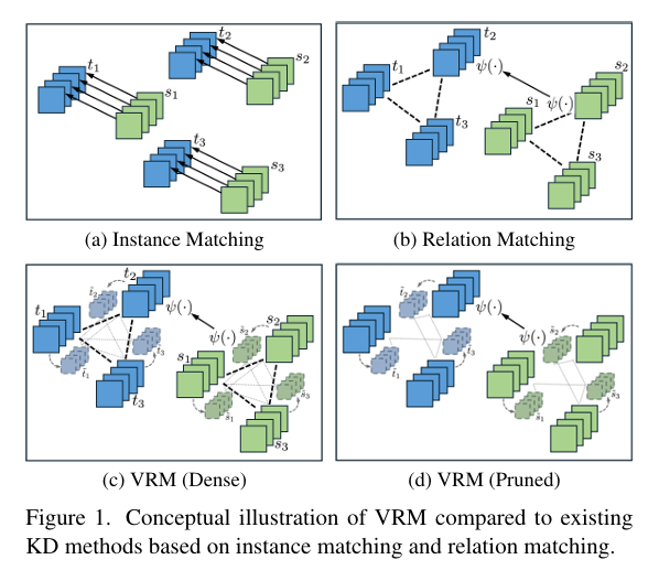
Introducing VRM: Virtual Relation Matching

To overcome these limitations, the authors propose Virtual Relation Matching (VRM)—a new paradigm in knowledge distillation that enriches relational learning with virtual views generated via data augmentation.

🔍 Core Idea:

Instead of relying solely on real sample relations, VRM constructs affinity graphs from both real and augmented (virtual) views, creating a denser, more diverse set of inter-sample, inter-class, and inter-view relationships.

This approach draws inspiration from self-supervised learning, where consistency between original and transformed views improves representation learning.

---

How VRM Works: A Step-by-Step Breakdown

Step 1: Generate Virtual Views

For each real image xi​ in a batch, apply semantic-preserving augmentations (e.g., rotation, color jitter, shear) to create a corresponding virtual view x~i​ . The paper uses RandAugment for this purpose.

Step 2: Extract Logits

Pass both real and virtual inputs through the teacher and student networks to obtain logits:

\[ \textbf{Teacher logits:} \quad z_t = f_t(x), \quad \tilde{z}_t = f_t(\tilde{x}) \] \[ \textbf{Student logits:} \quad z_s = f_s(x), \quad \tilde{z}_s = f_s(\tilde{x}) \]

Step 3: Construct Affinity Graphs

Build two types of relational graphs:

✅ Inter-Sample Relations (E_IS)

Measures similarity between sample representations:

\[ E_{m,n}^{\text{IS}} = \lVert z_m – z_n \rVert_2, \quad (z_m – z_n) \in \mathbb{R}^C \]

✅ Inter-Class Relations (E_IC)

Encodes class-level structure based on average logits per class.

These graphs now include three types of edges:

• Real–Real
• Virtual–Virtual
• Real–Virtual (new in VRM)

This inter-view relational knowledge significantly boosts generalization.

Step 4: Prune Spurious Edges

To combat noise and overfitting, VRM introduces a dynamic graph pruning mechanism that removes unreliable edges based on confidence thresholds.

This results in a sparse, robust graph that avoids propagating misleading gradients.

Step 5: Match Relations with Huber Loss

The final distillation loss minimizes the discrepancy between teacher and student relational graphs using the Huber loss:

\[ L_{\text{VRM}} = \phi(E_{S}^{IS}, E_{T}^{IS}) + \phi(E_{S}^{IC}, E_{T}^{IC}) \]

where ϕ(⋅) is the Huber loss function.

This makes VRM robust to outliers while preserving fine-grained relational structure.

---

Why VRM Outperforms Previous Methods

FEATURE	TRADITIONAL RM	VRM
Uses virtual views	❌	✅
Inter-view relations	❌	✅
Dynamic graph pruning	❌	✅
Susceptible to overfitting	High	Low
Gradient stability	Poor	High
Generalization to object detection	Limited	Strong

VRM’s advantages stem from its richer relational supervision, built-in regularization, and noise resistance—making it ideal for complex tasks like object detection and cross-architecture distillation.

---

Key Innovations in VRM

1. Inter-View Relations: A New Kind of Knowledge

VRM introduces inter-view relations—a previously unexplored form of relational knowledge that connects real and virtual samples. This allows the student to learn invariant patterns across transformations.

“Our designs are motivated by two important observations… RM methods are more susceptible to over-fitting than IM methods; RM methods are subject to an adverse gradient propagation effect.”

2. Compact Affinity Graphs with Rich Semantics

Unlike simple Gram matrices used in older RM methods, VRM uses normalized difference vectors to encode directional relationships between samples, capturing more discriminative information.

3. Dynamic Graph Pruning

By pruning low-confidence edges during training, VRM reduces overfitting and prevents gradient pollution from noisy predictions.

The paper shows this leads to smoother training dynamics and better validation performance.

---

Experimental Results: VRM Sets New SOTA

The authors evaluate VRM on CIFAR-100, ImageNet, and MS-COCO, comparing against over 30 KD methods including:

• Feature-based: FitNets, AT, NST, ReviewKD
• Logit-based: KD, DKD, LSKD
• Relation-based: RKD, CC, DIST

📊 Image Classification (CIFAR-100)

TEACHER→ STUDENT	METHOD	ACCURACY (%)
ResNet56 → DeiT-T	KD	73.25
ResNet56 → DeiT-T	LSKD	78.58
ResNet56 → DeiT-T	VRM	79.52✅

VRM improves DeiT-T by 14.44% over baseline with ResNet56 teacher.

📈 ImageNet (ResNet50 → MobileNetV2)

METHOD	TOP-1 ACCURACY
Previous SOTA	<74.0%
VRM	74.0%✅

This is the first time MobileNetV2 reaches 74.0% accuracy via distillation.

🔍 Object Detection (MS-COCO)

BACKBONE	METHOD	MAP (%)
R-50-FPN	FCFD	38.2
R-50-FPN	ReviewKD	38.1
R-50-FPN	VRM	37.9

While slightly behind top feature-based methods, VRM shows strong transferability to dense prediction tasks—a major win for relation-based KD.

---

VRM vs. Other KD Frameworks

FRAMEWORK	TYPE	REQUIRES TEACHER TRAINING ?	EXTRA PARAMETERS?	VIRTUAL VIEWS?
SSKD	Instance Matching	✅ (for pretext task)	✅	✅
HSAKD	Instance Matching	✅ (auxiliary classifiers)	✅	✅
VRM	Relation Matching	❌	❌	✅

✅ Key Advantage: VRM achieves superior performance without modifying the teacher architecture or adding auxiliary networks, making it simple, efficient, and plug-and-play.

---

Why VRM Matters for the Future of AI

As AI models grow larger, deploying them efficiently becomes critical. VRM offers a scalable, robust, and architecture-agnostic solution for knowledge transfer.

💡 Real-World Applications

• Edge AI: Deploy high-accuracy models on mobile phones.
• Autonomous Vehicles: Run fast detectors with minimal latency.
• Medical Imaging: Use compact models for real-time diagnosis.
• Green AI: Reduce carbon footprint by replacing large models.

Moreover, VRM’s success revives interest in relational reasoning—a capability essential for human-like intelligence.

---

Training Efficiency and Scalability

One concern with complex KD methods is computational overhead. But VRM is surprisingly efficient:

• No extra parameters
• No teacher retraining
• Lightweight graph construction
• Compatible with standard optimizers (SGD, AdamW)

From Table 10 in the paper:

“VRM is reasonably efficient compared to existing algorithms… does not introduce any extra overheads at inference.”

Additionally, the authors show that longer training (360 epochs) further boosts VRM’s performance, indicating its ability to scale with compute.

---

How to Implement VRM (Practical Tips)

Want to try VRM in your own projects? Here’s how:

1. Use RandAugment for Virtual Views

from torchvision import transforms
from torchvision.transforms.autoaugment import RandAugment

transform = transforms.Compose([
    RandAugment(),
    transforms.ToTensor(),
])

2. Compute Inter-Sample Relations

import torch.nn.functional as F

def inter_sample_relation(z1, z2):
    diff = z1.unsqueeze(1) - z2.unsqueeze(0)
    norm = diff.norm(dim=2, keepdim=True)
    return diff / (norm + 1e-8)

3. Apply Huber Loss for Matching

loss = F.huber_loss(student_graph, teacher_graph, delta=1.0)

For full implementation details, check the TorchSSL codebase referenced in the paper.

---

Conclusion: VRM Brings Relation-Based KD Back to the Forefront

Virtual Relation Matching (VRM) is not just another KD method—it’s a paradigm shift. By introducing inter-view relations, dynamic graph pruning, and compact affinity graphs, VRM solves long-standing issues in relation-based distillation.

It delivers state-of-the-art performance across image classification and object detection, without complex training pipelines or architectural changes.

Most importantly, VRM proves that relational knowledge, when properly harnessed, can outperform instance-level matching—opening new doors for future research in self-supervised distillation, cross-modal transfer, and robust representation learning.

---

Call to Action: Try VRM Today!

Are you working on model compression, edge AI, or efficient deep learning? Give VRM a try!

👉 Download the paper: arXiv:2502.20760
👉 Explore code: Check GitHub repositories like TorchSSL
👉 Run experiments: Apply VRM to your own teacher-student pairs

And if you found this article helpful, share it with your team, leave a comment, or subscribe for more cutting-edge AI insights!

Let’s make knowledge distillation smarter, faster, and more efficient—one virtual relation at a time.

Here is the complete code for the Virtual Relation Matching (VRM) loss function. You can integrate this class directly into your knowledge distillation training script.

# full_vrm_training_script.py

import torch
import torch.nn as nn
import torch.optim as optim
import torch.nn.functional as F
import torchvision
import torchvision.transforms as transforms
from torch.utils.data import DataLoader, Dataset
from tqdm import tqdm

# (Previously provided in the first response)
# Pasting the VRMLoss class here to make the script self-contained
class VRMLoss(nn.Module):
    """
    Implementation of the Virtual Relation Matching (VRM) loss from the paper:
    "VRM: Knowledge Distillation via Virtual Relation Matching"
    arXiv:2502.20760v3
    """
    def __init__(self, alpha: float, beta: float, ce_loss_on_real: bool = True, ce_loss_on_virtual: bool = True, unreliable_pruning_percentile: int = 30):
        super(VRMLoss, self).__init__()
        self.alpha = alpha
        self.beta = beta
        self.ce_loss_on_real = ce_loss_on_real
        self.ce_loss_on_virtual = ce_loss_on_virtual
        self.pruning_percentile = unreliable_pruning_percentile
        self.vrm_dist_loss = nn.HuberLoss(reduction='sum')
        self.ce_loss = nn.CrossEntropyLoss()

    def _get_relations(self, logits_real: torch.Tensor, logits_virtual: torch.Tensor):
        B, C = logits_real.shape
        z_r = logits_real.unsqueeze(1)
        z_v = logits_virtual.unsqueeze(0)
        diff_isv = z_r - z_v
        norm_isv = torch.linalg.norm(diff_isv, ord=2, dim=2, keepdim=True) + 1e-7
        E_isv = diff_isv / norm_isv
        
        w_r = logits_real.transpose(0, 1).unsqueeze(1)
        w_v = logits_virtual.transpose(0, 1).unsqueeze(0)
        diff_icv = w_r - w_v
        norm_icv = torch.linalg.norm(diff_icv, ord=2, dim=2, keepdim=True) + 1e-7
        E_icv = diff_icv / norm_icv
        return E_isv, E_icv

    def _unreliable_edge_pruning_mask(self, logits_real: torch.Tensor, logits_virtual: torch.Tensor):
        B, C = logits_real.shape
        probs_real = F.softmax(logits_real, dim=1)
        probs_virtual = F.softmax(logits_virtual, dim=1)
        
        p_r_isv = probs_real.unsqueeze(1)
        p_v_isv = probs_virtual.unsqueeze(0)
        joint_entropy_isv = -torch.sum(p_r_isv * torch.log(p_v_isv + 1e-7), dim=2)
        threshold_isv = torch.quantile(joint_entropy_isv, self.pruning_percentile / 100.0)
        isv_mask = (joint_entropy_isv <= threshold_isv)
        
        p_r_icv = probs_real.transpose(0, 1).unsqueeze(1)
        p_v_icv = probs_virtual.transpose(0, 1).unsqueeze(0)
        joint_entropy_icv = -torch.sum(p_r_icv * torch.log(p_v_icv + 1e-7), dim=2)
        threshold_icv = torch.quantile(joint_entropy_icv, self.pruning_percentile / 100.0)
        icv_mask = (joint_entropy_icv <= threshold_icv)
        return isv_mask, icv_mask

    def forward(self, logits_student_real, logits_student_virtual, logits_teacher_real, logits_teacher_virtual, labels):
        loss_ce = 0.0
        if self.ce_loss_on_real:
            loss_ce += self.ce_loss(logits_student_real, labels)
        if self.ce_loss_on_virtual:
            loss_ce += self.ce_loss(logits_student_virtual, labels)
            
        E_isv_t, E_icv_t = self._get_relations(logits_teacher_real.detach(), logits_teacher_virtual.detach())
        E_isv_s, E_icv_s = self._get_relations(logits_student_real, logits_student_virtual)
        
        isv_mask, icv_mask = self._unreliable_edge_pruning_mask(logits_student_real, logits_student_virtual)
        
        E_isv_s_pruned = E_isv_s * isv_mask.unsqueeze(-1)
        E_isv_t_pruned = E_isv_t * isv_mask.unsqueeze(-1)
        E_icv_s_pruned = E_icv_s * icv_mask.unsqueeze(-1)
        E_icv_t_pruned = E_icv_t * icv_mask.unsqueeze(-1)
        
        num_isv_edges = torch.sum(isv_mask) + 1e-7
        num_icv_edges = torch.sum(icv_mask) + 1e-7
        
        loss_isv = self.vrm_dist_loss(E_isv_s_pruned, E_isv_t_pruned) / num_isv_edges
        loss_icv = self.vrm_dist_loss(E_icv_s_pruned, E_icv_t_pruned) / num_icv_edges
        
        total_loss = loss_ce + self.alpha * loss_isv + self.beta * loss_icv
        return total_loss

# Custom Dataset to return two augmented views of an image
class DualViewDataset(Dataset):
    def __init__(self, dataset, transform_real, transform_virtual):
        self.dataset = dataset
        self.transform_real = transform_real
        self.transform_virtual = transform_virtual

    def __len__(self):
        return len(self.dataset)

    def __getitem__(self, idx):
        image, label = self.dataset[idx]
        real_view = self.transform_real(image)
        virtual_view = self.transform_virtual(image)
        return real_view, virtual_view, label

# Main training and evaluation functions
def train_one_epoch(teacher, student, loader, loss_fn, optimizer, device):
    teacher.eval()
    student.train()
    total_loss = 0.0
    
    progress_bar = tqdm(loader, desc="Training", leave=False)
    for real_view, virtual_view, labels in progress_bar:
        real_view, virtual_view, labels = real_view.to(device), virtual_view.to(device), labels.to(device)
        
        optimizer.zero_grad()
        
        # Get logits from both models for both views
        with torch.no_grad():
            logits_teacher_real = teacher(real_view)
            logits_teacher_virtual = teacher(virtual_view)
            
        logits_student_real = student(real_view)
        logits_student_virtual = student(virtual_view)
        
        # Calculate VRM loss
        loss = loss_fn(
            logits_student_real,
            logits_student_virtual,
            logits_teacher_real,
            logits_teacher_virtual,
            labels
        )
        
        loss.backward()
        optimizer.step()
        
        total_loss += loss.item()
        progress_bar.set_postfix(loss=loss.item())
        
    return total_loss / len(loader)

def validate(model, loader, device):
    model.eval()
    correct = 0
    total = 0
    with torch.no_grad():
        for images, labels in tqdm(loader, desc="Validating", leave=False):
            images, labels = images.to(device), labels.to(device)
            outputs = model(images)
            _, predicted = torch.max(outputs.data, 1)
            total += labels.size(0)
            correct += (predicted == labels).sum().item()
    return 100 * correct / total

def main():
    # --- 1. Configuration ---
    DEVICE = torch.device("cuda" if torch.cuda.is_available() else "cpu")
    NUM_CLASSES = 100 # For CIFAR-100
    BATCH_SIZE = 64
    LEARNING_RATE = 0.01
    MOMENTUM = 0.9
    WEIGHT_DECAY = 5e-4
    EPOCHS = 10 # Set to a higher number for full training
    
    # VRM Hyperparameters
    ALPHA = 800
    BETA = 400
    PRUNING_PERCENTILE = 30
    
    print(f"Using device: {DEVICE}")

    # --- 2. Data Preparation ---
    # Transformations for the "real" view (standard)
    transform_real = transforms.Compose([
        transforms.RandomCrop(32, padding=4),
        transforms.RandomHorizontalFlip(),
        transforms.ToTensor(),
        transforms.Normalize((0.5071, 0.4867, 0.4408), (0.2675, 0.2565, 0.2761)),
    ])

    # Transformations for the "virtual" view (strong augmentation via RandAugment)
    transform_virtual = transforms.Compose([
        transforms.RandAugment(),
        transforms.RandomCrop(32, padding=4),
        transforms.RandomHorizontalFlip(),
        transforms.ToTensor(),
        transforms.Normalize((0.5071, 0.4867, 0.4408), (0.2675, 0.2565, 0.2761)),
    ])
    
    # Standard transform for the validation set
    transform_val = transforms.Compose([
        transforms.ToTensor(),
        transforms.Normalize((0.5071, 0.4867, 0.4408), (0.2675, 0.2565, 0.2761)),
    ])
    
    # Load CIFAR-100 dataset
    train_base_dataset = torchvision.datasets.CIFAR100(root='./data', train=True, download=True)
    train_dataset = DualViewDataset(train_base_dataset, transform_real, transform_virtual)
    val_dataset = torchvision.datasets.CIFAR100(root='./data', train=False, download=True, transform=transform_val)
    
    train_loader = DataLoader(train_dataset, batch_size=BATCH_SIZE, shuffle=True, num_workers=4)
    val_loader = DataLoader(val_dataset, batch_size=BATCH_SIZE, shuffle=False, num_workers=4)

    # --- 3. Model Preparation ---
    # Load pre-trained teacher model (e.g., ResNet34)
    teacher = torchvision.models.resnet34(weights=torchvision.models.ResNet34_Weights.IMAGENET1K_V1)
    teacher.fc = nn.Linear(teacher.fc.in_features, NUM_CLASSES) # Adapt to CIFAR-100
    teacher = teacher.to(DEVICE)
    # Note: For best results, the teacher should be fine-tuned on CIFAR-100 first.
    # Here we use it directly for simplicity.
    
    # Load student model (e.g., MobileNetV2)
    student = torchvision.models.mobilenet_v2(weights=torchvision.models.MobileNet_V2_Weights.IMAGENET1K_V1)
    student.classifier[1] = nn.Linear(student.last_channel, NUM_CLASSES) # Adapt to CIFAR-100
    student = student.to(DEVICE)
    
    print("Teacher: ResNet34, Student: MobileNetV2")

    # --- 4. Training Setup ---
    loss_fn = VRMLoss(alpha=ALPHA, beta=BETA, unreliable_pruning_percentile=PRUNING_PERCENTILE)
    optimizer = optim.SGD(student.parameters(), lr=LEARNING_RATE, momentum=MOMENTUM, weight_decay=WEIGHT_DECAY)
    scheduler = optim.lr_scheduler.CosineAnnealingLR(optimizer, T_max=EPOCHS)
    
    # --- 5. Training and Evaluation Loop ---
    best_acc = 0.0
    for epoch in range(EPOCHS):
        print(f"\n--- Epoch {epoch+1}/{EPOCHS} ---")
        avg_loss = train_one_epoch(teacher, student, train_loader, loss_fn, optimizer, DEVICE)
        val_acc = validate(student, val_loader, DEVICE)
        scheduler.step()
        
        print(f"Epoch {epoch+1} Summary: Avg Loss = {avg_loss:.4f}, Validation Acc = {val_acc:.2f}%")
        
        if val_acc > best_acc:
            best_acc = val_acc
            print(f"✨ New best accuracy! Saving model to 'student_best.pth'")
            torch.save(student.state_dict(), 'student_best.pth')

    print(f"\nTraining finished. Best student accuracy: {best_acc:.2f}%")

if __name__ == '__main__':
    main()

Related posts, You May like to read

1. 7 Shocking Truths About Knowledge Distillation: The Good, The Bad, and The Breakthrough (SAKD)
2. 7 Revolutionary Breakthroughs in Medical Image Translation (And 1 Fatal Flaw That Could Derail Your AI Model)
3. DeepSPV: Revolutionizing 3D Spleen Volume Estimation from 2D Ultrasound with AI
4. ACAM-KD: Adaptive and Cooperative Attention Masking for Knowledge Distillation
5. GeoSAM2 3D Part Segmentation — Prompt-Controllable, Geometry-Aware Masks for Precision 3D Editing
6. Enhancing Vision-Audio Capability in Omnimodal LLMs with Self-KD