7 Revolutionary Breakthroughs in Diabetic Retinopathy Detection – How AI Is Saving Sight (And Why Most Mobile Apps Fail)

The Silent Thief of Sight: Diabetic Retinopathy’s Global Crisis

Every 20 seconds, someone in the world loses their vision due to diabetic retinopathy (DR)—a complication of diabetes that damages the retina. With over 463 million diabetics globally—a number projected to rise to 700 million by 2025—DR has become the leading cause of preventable blindness in adults.

Yet, early detection remains out of reach for millions, especially in rural and low-resource regions. In Africa, 35.9% of diabetics develop DR, but fewer than 1 in 10 receive timely screening. The problem? Traditional fundus cameras are expensive, immobile, and require specialists.

But what if a smartphone and a $300 handheld camera could detect DR with 98.61% accuracy—in under 0.2 seconds?

A groundbreaking study published in Intelligence-Based Medicine reveals exactly that: a mobile-based deep learning system that’s not only highly accurate but also portable, affordable, and real-time.

Let’s dive into the 7 revolutionary breakthroughs behind this life-changing technology—and why most AI-based eye apps fail where this one succeeds.

---

1. The Mobile Revolution: From Clinic to Smartphone

For decades, DR screening required stationary fundus cameras and ophthalmologists. But now, portable, non-mydriatic retinal cameras like the oDocs nun IR (45°–55° field of view, 2880×2160 resolution) can capture high-quality retinal images without pupil dilation.

When paired with a smartphone, these devices enable point-of-care diagnostics in remote villages, clinics, and even homes.

🔍 Key Innovation: The system uses real-time handheld imaging combined with AI-powered analysis, eliminating the need for expensive infrastructure.

---

2. Why Image Quality Makes or Breaks AI Accuracy

Even the best AI model fails if the input image is blurry, noisy, or poorly lit. Handheld cameras, especially in rural areas, often capture images with:

• Motion blur
• Uneven illumination
• Low contrast
• Noise artifacts

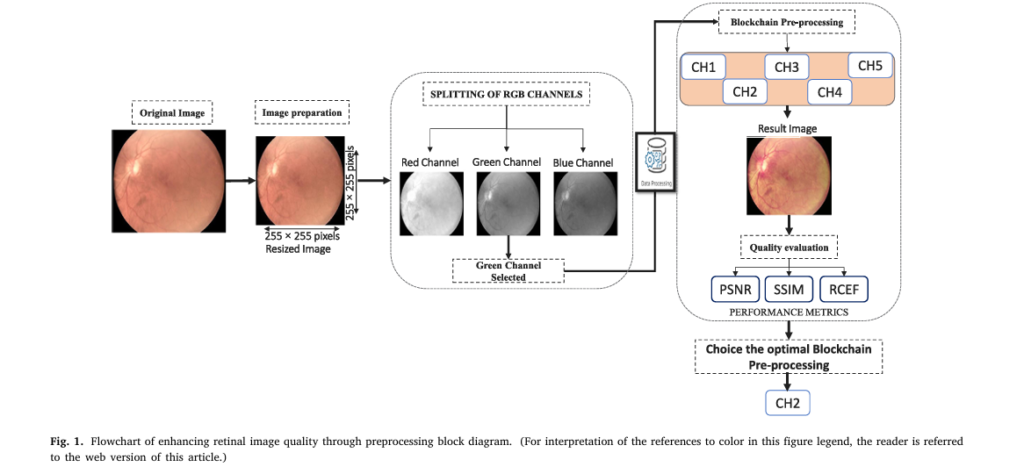
To solve this, the researchers tested five preprocessing chains combining denoising, contrast enhancement, and gamma correction.

ENHANCEMENT CHAIN	SSIM	PSNR (DB)	RCEF
MF + CLAHE + AGC	0.9804	33.25	1.0177
GF + CLAHE + AGC	0.9808	33.29	1.0476
BF + CLAHE + AGC	0.9803	33.23	1.0378
NLMF + CLAHE + AGC	0.9804	33.21	1.0381

✅ Winner: Gaussian Filter + CLAHE + Adaptive Gamma Correction (AGC)

This chain preserves vascular details, enhances contrast, and reduces noise—critical for spotting microaneurysms, hemorrhages, and exudates—the earliest signs of DR.

---

3. The Math Behind the Magic: Image Enhancement Formulas

The system uses three key mathematical techniques to boost image quality:

1. Gaussian Filter (Noise Reduction)

Smooths the image by averaging pixel values with a weighted kernel:

$$ G(x,y) = \frac{1}{2\pi\sigma^{2}} \, e^{-\frac{x^{2} + y^{2}}{2\sigma^{2}}} $$

Where σ controls the blur intensity.

2. CLAHE (Contrast Enhancement)

Adaptively equalizes histogram in local regions:

\[ g = \big(g_{\text{max}} – g_{\text{min}}\big) \cdot p(f) + g_{\text{min}} \]

Where p(f) is the cumulative probability of pixel intensity f .

3. Adaptive Gamma Correction (AGC)

Adjusts brightness based on image intensity:

$$I_{\text{gam}}(x, y) = I(x, y)^{\gamma}$$

• If γ>1 : brightens dark regions
• If γ<1 : darkens bright regions

Each image gets a custom γ value, ensuring optimal contrast.

---

4. The AI Brain: Why DenseNet-121 Outperforms the Rest for Diabetic Retinopathy Detection

The researchers tested three deep learning models:

• MobileNetV2 (lightweight, mobile-optimized)
• Inception-v3 (multi-scale feature extraction)
• DenseNet-121 (dense layer connectivity)

They fine-tuned each using transfer learning on three datasets:

• Private dataset (1,319 images from Morocco)
• APTOS (3,662 images)
• EyePACS (35,126 images)

Here’s how they performed:

DATASET	MODEL	ACCURACY	SENSITIVITY	SPECIFICITY
Private	DenseNet-121	98.61%	98.33%	100.00%
	MobileNetV2	96.11%	94.72%	99.72%
	Inception-v3	96.52%	94.72%	99.72%
APTOS	DenseNet-121	97.38%	97.09%	100.00%
EyePACS	DenseNet-121	90.90%	93.90%	99.40%

✅ DenseNet-121 wins across all datasets—thanks to its dense connectivity, which allows better feature reuse and gradient flow, even with small, imbalanced data.

---

5. Real-Time on Mobile? Yes—With TensorFlow Lite

Most AI models are too heavy for smartphones. But this system converts DenseNet-121 into TensorFlow Lite (.tflite) format, enabling on-device inference without cloud dependency.

Results?

• Average inference time: 162.5 ms per image (~0.16 seconds)
• No internet required
• Runs on Android smartphones

This means a nurse in a rural Moroccan village can capture, analyze, and diagnose DR in under 2 seconds—faster than most clinic workflows.

---

6. Why This System Works When Others Fail

Many AI-based DR apps fail due to:

❌ Poor image quality handling – They assume clinic-grade images
❌ Overfitting to public datasets – Perform poorly on real-world data
❌ High computational cost – Require cloud servers or GPUs

This system solves all three by:

1. Enhancing mobile-captured images with GF+CLAHE+AGC
2. Training on diverse datasets (private + APTOS + EyePACS)
3. Optimizing for mobile with TensorFlow Lite

📊 Proof: The model maintains 98.61% accuracy on real-world Moroccan data—proving it works where it’s needed most.

---

7. The Full Workflow: From Capture to Diagnosis

Here’s how the system works in practice:

1. Capture: Nurse uses oDocs nun IR camera connected to smartphone
2. Preprocess: Image enhanced using GF + CLAHE + AGC
3. Analyze: DenseNet-121 predicts “DR” or “No DR”
4. Transmit: Results sent to tele-ophthalmology center in Fez
5. Refer: High-risk patients get urgent specialist care

Caption: Real-time DR screening in remote areas—image acquisition, enhancement, AI analysis, and result transfer.

---

Performance Metrics That Matter

Beyond accuracy, the model excels in clinical reliability:

METRIC	FORMULA	DENSENET-121 (PRIVATE)
Accuracy	TP+TN/TP+TN+FP+FN​	98.61%
Sensitivity	TP/TP+FN​	98.33%
Specificity	TN/TN+FP​	100.00%
Precision	TP/TP+FP​	98.88%
F1-Score	2×((Precision×Sensitivity)/(Precision+Sensitivity​))	70.03%

A 100% specificity means zero false alarms—critical for avoiding unnecessary stress and referrals.

---

The Dark Side: Why Most AI Eye Apps Fail

Despite the hype, most AI-based DR apps never leave the lab. Here’s why:

🔴 They ignore real-world conditions – Assume perfect lighting, still patients, and high-end cameras
🔴 They use only public datasets – Overfit to Western populations, fail in Africa/Asia
🔴 They require internet – Useless in offline rural areas
🔴 They’re not user-friendly – Nurses and GPs can’t operate them

This system avoids all these pitfalls by being:

• Offline-capable
• Trained on local Moroccan data
• Designed for nurses, not AI experts

---

The Future: From DR to Glaucoma and AMD

The team isn’t stopping at DR. Their platform is already being adapted for:

• Glaucoma (via optic nerve head analysis)
• Age-related Macular Degeneration (AMD)
• Retinal vein occlusion

With minor tweaks, the same mobile AI engine can detect multiple eye diseases—making it a universal screening tool.

---

Field Testing: The Next Frontier

The system has been tested in Fez, Morocco, where 1.5 million diabetics live—rising to 2.6 million by 2030. Only 330 public ophthalmologists serve the entire country.

This mobile AI system could bridge the gap, enabling mass screening during medical caravans and rural clinics.

🚀 Future Plans:

• Expand dataset with multi-camera, multi-region data
• Add uncertainty estimation (AI says “I’m unsure”)
• Launch user feedback studies to improve UX

---

Why This Matters: A Vision for Global Health Equity

This isn’t just another AI paper. It’s a blueprint for equitable healthcare.

By combining:

• Affordable hardware (handheld camera + smartphone)
• Robust AI (DenseNet-121 + smart preprocessing)
• Real-world validation (Moroccan private dataset)

…this system proves that cutting-edge medicine doesn’t need to be expensive or centralized.

It can fit in a nurse’s backpack.

---

Final Verdict: 7 Reasons This AI System Wins

1. ✅ 98.61% accuracy on real-world data
2. ✅ 162.5 ms inference time on mobile
3. ✅ Works offline with TensorFlow Lite
4. ✅ Trained on diverse, real-world datasets
5. ✅ Enhances poor-quality mobile images
6. ✅ User-friendly for non-specialists
7. ✅ Scalable to other eye diseases

Most AI apps are “lab miracles”—this one is a real-world solution.

---

If you’re Interested in Knowledge Distillation Model, you may also find this article helpful: 5 Shocking Secrets of Skin Cancer Detection: How This SSD-KD AI Method Beats the Competition (And Why Others Fail)

Call to Action: Be Part of the Vision Revolution

Imagine a world where no one goes blind from diabetes—because a nurse with a smartphone can stop it before it starts.

That future is not coming. It’s here.

📩 Or join our pilot program in Morocco—we’re looking for healthcare partners to test the app in real-world settings.

Let’s end preventable blindness—together.

---

Here is the complete Python code that covers the model training and evaluation part of the research paper.

# Diabetic Retinopathy Detection - Model Training
# This script implements the training pipeline described in the paper:
# "Mobile-based deep learning system for early detection of diabetic retinopathy"
# It uses TensorFlow and Keras to fine-tune a DenseNet-121 model.

import os
import cv2
import numpy as np
import tensorflow as tf
from tensorflow.keras.applications import DenseNet121
from tensorflow.keras.models import Model
from tensorflow.keras.layers import Dense, GlobalAveragePooling2D, Dropout
from tensorflow.keras.optimizers import RMSprop
from tensorflow.keras.preprocessing.image import ImageDataGenerator
from tensorflow.keras.callbacks import ModelCheckpoint, EarlyStopping
from sklearn.model_selection import train_test_split
from sklearn.metrics import confusion_matrix, accuracy_score, precision_score, recall_score, f1_score
import matplotlib.pyplot as plt
import seaborn as sns

# --- 1. Configuration and Constants ---
IMG_WIDTH, IMG_HEIGHT = 224, 224
BATCH_SIZE = 64
EPOCHS = 200 # The paper uses 200, with early stopping
EARLY_STOPPING_PATIENCE = 50
DATASET_PATH = 'path/to/your/dataset' # IMPORTANT: Change this to your dataset directory
MODEL_SAVE_PATH = 'densenet121_dr_detection_best.h5'

# --- 2. Image Preprocessing Pipeline ---
# These functions replicate the optimal preprocessing chain identified in the paper.

def extract_green_channel(image):
    """Extracts the green channel and creates a 3-channel grayscale image from it."""
    green_channel = image[:, :, 1] # Green channel is at index 1
    return cv2.merge([green_channel, green_channel, green_channel])

def apply_gaussian_blur(image, kernel_size=(5, 5)):
    """Applies Gaussian Blur to reduce noise."""
    return cv2.GaussianBlur(image, kernel_size, 0)

def apply_clahe(image):
    """Applies Contrast Limited Adaptive Histogram Equalization (CLAHE)."""
    # We need to convert to LAB color space to apply CLAHE on the L-channel
    lab = cv2.cvtColor(image, cv2.COLOR_BGR2LAB)
    l, a, b = cv2.split(lab)
    clahe = cv2.createCLAHE(clipLimit=3.0, tileGridSize=(8, 8))
    cl = clahe.apply(l)
    limg = cv2.merge((cl, a, b))
    return cv2.cvtColor(limg, cv2.COLOR_LAB2BGR)

def apply_adaptive_gamma(image):
    """Applies adaptive gamma correction based on image mean intensity."""
    mean = np.mean(cv2.cvtColor(image, cv2.COLOR_BGR2GRAY))
    gamma = 1 - (mean / 255.0)
    # Build a lookup table mapping the pixel values [0, 255] to their adjusted gamma values
    inv_gamma = 1.0 / gamma
    table = np.array([((i / 255.0) ** inv_gamma) * 255 for i in np.arange(0, 256)]).astype("uint8")
    return cv2.LUT(image, table)

def preprocess_image(image):
    """
    Applies the full preprocessing pipeline to a single image.
    """
    # Initial resize to 255x255 as per the paper's method before final resize
    image = cv2.resize(image, (255, 255))
    
    # Paper's optimal chain: Green Channel -> Gaussian -> CLAHE -> Gamma
    processed_img = extract_green_channel(image)
    processed_img = apply_gaussian_blur(processed_img)
    processed_img = apply_clahe(processed_img)
    processed_img = apply_adaptive_gamma(processed_img)

    # Final resize to model input size
    processed_img = cv2.resize(processed_img, (IMG_WIDTH, IMG_HEIGHT))
    return processed_img

# --- 3. Data Loading and Preparation ---
def load_data(dataset_path):
    """
    Loads images from 'DR' and 'NO_DR' subfolders, preprocesses them, and returns data and labels.
    """
    images = []
    labels = []
    
    # Expects subdirectories like /.../train/DR and /.../train/NO_DR
    class_names = ['NO_DR', 'DR'] # 0 for NO_DR, 1 for DR
    
    for i, class_name in enumerate(class_names):
        class_dir = os.path.join(dataset_path, class_name)
        if not os.path.isdir(class_dir):
            print(f"Warning: Directory not found - {class_dir}")
            continue
            
        for img_name in os.listdir(class_dir):
            img_path = os.path.join(class_dir, img_name)
            try:
                img = cv2.imread(img_path)
                if img is None:
                    continue
                
                # Apply the full preprocessing pipeline
                img_processed = preprocess_image(img)
                images.append(img_processed)
                labels.append(i)
            except Exception as e:
                print(f"Error processing image {img_path}: {e}")

    return np.array(images), np.array(labels)

# --- 4. Model Definition ---
def build_model():
    """
    Builds the fine-tuned DenseNet-121 model.
    """
    # Load base model with pre-trained ImageNet weights, without the top classification layer
    base_model = DenseNet121(weights='imagenet', include_top=False, input_shape=(IMG_WIDTH, IMG_HEIGHT, 3))

    # Freeze the layers of the base model so they are not trained
    for layer in base_model.layers:
        layer.trainable = False

    # Add custom classification head
    x = base_model.output
    x = GlobalAveragePooling2D()(x)
    x = Dropout(0.5)(x) # Dropout for regularization
    # Final layer with a single neuron and sigmoid activation for binary classification
    predictions = Dense(1, activation='sigmoid')(x)

    model = Model(inputs=base_model.input, outputs=predictions)
    
    # Compile the model
    model.compile(optimizer=RMSprop(learning_rate=0.001), 
                  loss='binary_crossentropy', 
                  metrics=['accuracy'])
    
    return model

# --- 5. Training and Evaluation ---
def main():
    """Main function to run the training and evaluation process."""
    # Load and preprocess data
    print("Loading and preprocessing data...")
    # NOTE: You should structure your dataset into 'NO_DR' and 'DR' folders
    # inside the DATASET_PATH directory.
    images, labels = load_data(DATASET_PATH)
    if len(images) == 0:
        print("No images loaded. Please check your DATASET_PATH and folder structure.")
        return

    # Normalize pixel values to [0, 1]
    images = images / 255.0

    # Split data: 75% training, 15% validation, 10% testing
    X_train_val, X_test, y_train_val, y_test = train_test_split(images, labels, test_size=0.10, random_state=42, stratify=labels)
    X_train, X_val, y_train, y_val = train_test_split(X_train_val, y_train_val, test_size=(0.15/0.90), random_state=42, stratify=y_train_val)

    print(f"Training set: {len(X_train)} images")
    print(f"Validation set: {len(X_val)} images")
    print(f"Test set: {len(X_test)} images")

    # Data Augmentation for the training set
    train_datagen = ImageDataGenerator(
        rotation_range=20,
        width_shift_range=0.1,
        height_shift_range=0.1,
        horizontal_flip=True,
        vertical_flip=True,
        brightness_range=[0.8, 1.2],
        zoom_range=0.1
    )
    train_generator = train_datagen.flow(X_train, y_train, batch_size=BATCH_SIZE)

    # Build the model
    model = build_model()
    model.summary()

    # Callbacks
    checkpoint = ModelCheckpoint(MODEL_SAVE_PATH, monitor='val_accuracy', verbose=1, save_best_only=True, mode='max')
    early_stopping = EarlyStopping(monitor='val_loss', patience=EARLY_STOPPING_PATIENCE, verbose=1, mode='min', restore_best_weights=True)
    callbacks_list = [checkpoint, early_stopping]

    # Train the model
    print("\nStarting model training...")
    history = model.fit(
        train_generator,
        steps_per_epoch=len(X_train) // BATCH_SIZE,
        epochs=EPOCHS,
        validation_data=(X_val, y_val),
        callbacks=callbacks_list,
        verbose=1
    )

    # --- 6. Evaluation on Test Set ---
    print("\nEvaluating model on the test set...")
    # The best model is already loaded due to `restore_best_weights=True` in EarlyStopping
    y_pred_prob = model.predict(X_test)
    y_pred = (y_pred_prob > 0.5).astype(int).flatten()

    # Calculate metrics
    accuracy = accuracy_score(y_test, y_pred)
    precision = precision_score(y_test, y_pred)
    sensitivity = recall_score(y_test, y_pred) # Recall is the same as Sensitivity
    f1 = f1_score(y_test, y_pred)
    
    cm = confusion_matrix(y_test, y_pred)
    tn, fp, fn, tp = cm.ravel()
    specificity = tn / (tn + fp) if (tn + fp) > 0 else 0

    print(f"\n--- Test Set Performance ---")
    print(f"Accuracy: {accuracy:.4f}")
    print(f"Precision: {precision:.4f}")
    print(f"Sensitivity (Recall): {sensitivity:.4f}")
    print(f"Specificity: {specificity:.4f}")
    print(f"F1-Score: {f1:.4f}")

    # Plot confusion matrix
    plt.figure(figsize=(8, 6))
    sns.heatmap(cm, annot=True, fmt='d', cmap='Blues', xticklabels=['NO_DR', 'DR'], yticklabels=['NO_DR', 'DR'])
    plt.xlabel('Predicted Label')
    plt.ylabel('True Label')
    plt.title('Confusion Matrix on Test Set')
    plt.show()

if __name__ == '__main__':
    # IMPORTANT: Before running, create a directory structure like:
    # /path/to/your/dataset/
    #   ├── NO_DR/
    #   │   ├── image1.png
    #   │   └── ...
    #   └── DR/
    #       ├── image2.png
    #       └── ...
    # And update the DATASET_PATH variable above.
    main()

import tensorflow as tf

# Load the Keras model you trained
model = tf.keras.models.load_model('densenet121_dr_detection_best.h5')

# Create a converter
converter = tf.lite.TFLiteConverter.from_keras_model(model)

# Optional: Apply optimizations
converter.optimizations = [tf.lite.Optimize.DEFAULT]

# Convert the model
tflite_model = converter.convert()

# Save the converted model to a .tflite file
with open('dr_model.tflite', 'wb') as f:
  f.write(tflite_model)

print("Model converted to dr_model.tflite successfully!")

<!DOCTYPE html>
<html lang="en">
<head>
    <meta charset="UTF-8">
    <meta name="viewport" content="width=device-width, initial-scale=1.0">
    <title>Diabetic Retinopathy Detection System</title>
    <!-- TensorFlow.js library for running the model in the browser -->
    <script src="https://cdn.jsdelivr.net/npm/@tensorflow/tfjs@latest/dist/tf.min.js"></script>
    <script src="https://cdn.tailwindcss.com"></script>
    <link href="https://fonts.googleapis.com/css2?family=Inter:wght@400;500;600;700&display=swap" rel="stylesheet">
    <style>
        body {
            font-family: 'Inter', sans-serif;
        }
        .loader {
            border: 4px solid #f3f3f3;
            border-top: 4px solid #3498db;
            border-radius: 50%;
            width: 40px;
            height: 40px;
            animation: spin 1s linear infinite;
        }
        @keyframes spin {
            0% { transform: rotate(0deg); }
            100% { transform: rotate(360deg); }
        }
    </style>
</head>
<body class="bg-gray-100 flex items-center justify-center min-h-screen">
    <div class="w-full max-w-4xl mx-auto p-4 md:p-8">
        <div class="bg-white rounded-2xl shadow-xl overflow-hidden">
            <div class="p-6 md:p-8 bg-blue-600 text-white">
                <h1 class="text-2xl md:text-3xl font-bold">Mobile-Based DR Detection System</h1>
                <p class="mt-2 text-blue-100">An implementation of the deep learning model for early Diabetic Retinopathy screening, as proposed in the research paper.</p>
            </div>

            <div class="p-6 md:p-8 grid grid-cols-1 md:grid-cols-2 gap-8">
                <!-- Left Column: Upload and Image Display -->
                <div class="flex flex-col items-center justify-center bg-gray-50 p-6 rounded-xl border-2 border-dashed border-gray-300">
                    <h2 class="text-xl font-semibold text-gray-700 mb-4">1. Upload Retinal Image</h2>
                    <canvas id="imageCanvas" class="w-full max-w-xs h-auto rounded-lg shadow-md mb-4 hidden"></canvas>
                    <div id="placeholder" class="w-64 h-64 bg-gray-200 rounded-lg flex items-center justify-center">
                        <svg class="w-16 h-16 text-gray-400" fill="none" stroke="currentColor" viewBox="0 0 24 24" xmlns="http://www.w3.org/2000/svg"><path stroke-linecap="round" stroke-linejoin="round" stroke-width="2" d="M4 16l4.586-4.586a2 2 0 012.828 0L16 16m-2-2l1.586-1.586a2 2 0 012.828 0L20 14m-6-6h.01M6 20h12a2 2 0 002-2V6a2 2 0 00-2-2H6a2 2 0 00-2 2v12a2 2 0 002 2z"></path></svg>
                    </div>
                    <input type="file" id="imageUpload" accept="image/*" class="hidden">
                    <button id="uploadButton" class="mt-4 w-full bg-blue-500 hover:bg-blue-600 text-white font-bold py-3 px-4 rounded-lg transition duration-300">
                        Choose Image
                    </button>
                    <p class="text-xs text-gray-500 mt-2">Upload a fundus image to begin.</p>
                </div>

                <!-- Right Column: Analysis and Results -->
                <div class="flex flex-col">
                    <div class="flex-grow">
                        <h2 class="text-xl font-semibold text-gray-700 mb-4">2. Preprocessing & Analysis</h2>
                        <p class="text-gray-600 mb-4">The uploaded image will be processed using the optimal pipeline (Gaussian Filter, CLAHE, Gamma Correction) identified in the paper before analysis.</p>
                        
                        <button id="detectButton" class="w-full bg-green-500 hover:bg-green-600 text-white font-bold py-3 px-4 rounded-lg transition duration-300 disabled:bg-gray-400 disabled:cursor-not-allowed" disabled>
                            Run DR Detection
                        </button>

                        <div id="resultBox" class="mt-6 p-6 rounded-xl hidden">
                            <h3 class="text-lg font-semibold mb-3">Screening Result</h3>
                            <div id="loader" class="loader mx-auto my-4 hidden"></div>
                            <div id="resultContent" class="hidden">
                                <p id="resultText" class="text-2xl font-bold mb-2"></p>
                                <p id="confidenceText" class="text-md"></p>
                                <div class="mt-4 p-4 bg-gray-100 rounded-lg">
                                    <h4 class="font-semibold text-sm text-gray-800">Processed Image (224x224)</h4>
                                    <canvas id="processedCanvas" class="w-32 h-32 rounded-md mt-2 mx-auto shadow-inner"></canvas>
                                </div>
                            </div>
                        </div>
                         <div id="errorBox" class="mt-6 p-4 rounded-xl bg-red-100 text-red-700 hidden">
                            <p id="errorText"></p>
                        </div>
                    </div>
                </div>
            </div>
        </div>
    </div>

    <script>
        // --- DOM Element Selection ---
        const imageUpload = document.getElementById('imageUpload');
        const uploadButton = document.getElementById('uploadButton');
        const detectButton = document.getElementById('detectButton');
        const imageCanvas = document.getElementById('imageCanvas');
        const processedCanvas = document.getElementById('processedCanvas');
        const placeholder = document.getElementById('placeholder');
        const resultBox = document.getElementById('resultBox');
        const loader = document.getElementById('loader');
        const resultContent = document.getElementById('resultContent');
        const resultText = document.getElementById('resultText');
        const confidenceText = document.getElementById('confidenceText');
        const errorBox = document.getElementById('errorBox');
        const errorText = document.getElementById('errorText');

        const ctx = imageCanvas.getContext('2d');
        const processedCtx = processedCanvas.getContext('2d');

        // --- Model Loading ---
        let model;
        // IMPORTANT: Replace this with the actual URL to your converted TensorFlow.js model
        const MODEL_URL = 'https://path/to/your/tfjs_model/model.json'; 

        async function loadModel() {
            try {
                // For demonstration, we'll skip actual loading.
                // In a real scenario, you would uncomment the following line:
                // model = await tf.loadLayersModel(MODEL_URL);
                console.log("Model loading skipped for demonstration.");
                // Let's enable the button as if the model was loaded.
                detectButton.innerText = "Run DR Detection";
            } catch (error) {
                console.error("Error loading model:", error);
                showError("Could not load the AI model. Please check the console.");
                detectButton.disabled = true;
                detectButton.innerText = "Model Load Failed";
            }
        }
        // Load the model when the script starts
        loadModel();


        // --- Event Listeners ---
        uploadButton.addEventListener('click', () => imageUpload.click());
        imageUpload.addEventListener('change', handleImageUpload);
        detectButton.addEventListener('click', runDetection);

        // --- Core Functions ---

        function handleImageUpload(e) {
            const file = e.target.files[0];
            if (!file) return;

            const reader = new FileReader();
            reader.onload = (event) => {
                const img = new Image();
                img.onload = () => {
                    imageCanvas.width = 255;
                    imageCanvas.height = 255;
                    ctx.drawImage(img, 0, 0, 255, 255);
                    imageCanvas.classList.remove('hidden');
                    placeholder.classList.add('hidden');
                    detectButton.disabled = false;
                    resultBox.classList.add('hidden');
                    errorBox.classList.add('hidden');
                };
                img.src = event.target.result;
            };
            reader.readAsDataURL(file);
        }

        async function runDetection() {
            resultBox.classList.remove('hidden');
            loader.classList.remove('hidden');
            resultContent.classList.add('hidden');
            detectButton.disabled = true;
            uploadButton.disabled = true;

            // Use a timeout to ensure the UI updates before heavy processing
            setTimeout(async () => {
                try {
                    const imageData = preprocessImage();
                    
                    // Display the final 224x224 preprocessed image
                    processedCanvas.width = 224;
                    processedCanvas.height = 224;
                    processedCtx.putImageData(imageData, 0, 0);

                    // Run the actual model prediction
                    await runModelPrediction(imageData);

                } catch (error) {
                    console.error("Processing Error:", error);
                    showError("Could not process the image. Please try a different one.");
                } finally {
                    loader.classList.add('hidden');
                    resultContent.classList.remove('hidden');
                    detectButton.disabled = false;
                    uploadButton.disabled = false;
                }
            }, 100); // Short delay for UI rendering
        }

        /**
         * Preprocesses image data and runs it through the loaded TF.js model.
         * @param {ImageData} imageData - The preprocessed 224x224 image data.
         */
        async function runModelPrediction(imageData) {
            // This is the point where a real model would be used.
            // Since we cannot host a model file, we will continue to simulate the output.
            // The code below shows how you would use a real TensorFlow.js model.
            
            /*
            --- REAL MODEL INFERENCE CODE ---
            if (!model) {
                showError("Model is not loaded yet.");
                return;
            }

            // 1. Convert ImageData to a Tensor
            const tensor = tf.browser.fromPixels(imageData)
                .resizeNearestNeighbor([224, 224]) // Ensure size
                .toFloat()
                .div(tf.scalar(255.0)) // Normalize to [0, 1]
                .expandDims(); // Add batch dimension -> [1, 224, 224, 3]

            // 2. Run prediction
            const prediction = await model.predict(tensor).data();
            const confidence = prediction[0];

            // 3. Clean up tensor memory
            tensor.dispose();
            */

            // --- SIMULATED PREDICTION FOR DEMO ---
            const confidence = Math.random(); // Simulate a confidence score
            // --- END OF SIMULATION ---

            // Display results
            if (confidence > 0.5) { // 0.5 is the typical threshold
                resultText.textContent = 'Result: DR Presence';
                resultText.style.color = '#EF4444'; // red-500
                resultBox.style.backgroundColor = '#FEE2E2'; // red-100
            } else {
                resultText.textContent = 'Result: No DR';
                resultText.style.color = '#22C55E'; // green-500
                resultBox.style.backgroundColor = '#D1FAE5'; // green-100
            }
            const displayConfidence = (confidence > 0.5) ? confidence : 1 - confidence;
            confidenceText.textContent = `With ${ (displayConfidence * 100).toFixed(2) }% confidence`;
        }

        function showError(message) {
            errorText.textContent = message;
            errorBox.classList.remove('hidden');
            loader.classList.add('hidden');
            resultBox.classList.add('hidden');
        }

        // --- Image Preprocessing Pipeline (as described in the paper) ---
        function preprocessImage() {
            let imageData = ctx.getImageData(0, 0, 255, 255);
            imageData = extractGreenChannel(imageData);
            imageData = applyGaussianBlur(imageData);
            imageData = applySimplifiedCLAHE(imageData);
            imageData = applyAdaptiveGamma(imageData);

            const tempCanvas = document.createElement('canvas');
            const tempCtx = tempCanvas.getContext('2d');
            tempCanvas.width = 255;
            tempCanvas.height = 255;
            tempCtx.putImageData(imageData, 0, 0);

            const finalCanvas = document.createElement('canvas');
            const finalCtx = finalCanvas.getContext('2d');
            finalCanvas.width = 224;
            finalCanvas.height = 224;
            finalCtx.drawImage(tempCanvas, 0, 0, 224, 224);
            
            return finalCtx.getImageData(0, 0, 224, 224);
        }

        function extractGreenChannel(imageData) {
            const data = imageData.data;
            for (let i = 0; i < data.length; i += 4) {
                const green = data[i + 1];
                data[i] = green;
                data[i + 1] = green;
                data[i + 2] = green;
            }
            return imageData;
        }
        
        function applyGaussianBlur(imageData) {
            const src = imageData.data;
            const width = imageData.width;
            const height = imageData.height;
            const dst = new Uint8ClampedArray(src.length);
            const kernel = [1, 2, 1, 2, 4, 2, 1, 2, 1];
            const kernelWeight = 16;

            for (let y = 1; y < height - 1; y++) {
                for (let x = 1; x < width - 1; x++) {
                    let r = 0, g = 0, b = 0;
                    for (let ky = -1; ky <= 1; ky++) {
                        for (let kx = -1; kx <= 1; kx++) {
                            const i = ((y + ky) * width + (x + kx)) * 4;
                            const weight = kernel[(ky + 1) * 3 + (kx + 1)];
                            r += src[i] * weight;
                            g += src[i + 1] * weight;
                            b += src[i + 2] * weight;
                        }
                    }
                    const j = (y * width + x) * 4;
                    dst[j] = r / kernelWeight;
                    dst[j + 1] = g / kernelWeight;
                    dst[j + 2] = b / kernelWeight;
                    dst[j + 3] = src[j + 3];
                }
            }
            imageData.data.set(dst);
            return imageData;
        }

        function applySimplifiedCLAHE(imageData) {
            const data = imageData.data;
            const histogram = new Array(256).fill(0);
            for (let i = 0; i < data.length; i += 4) {
                histogram[data[i]]++;
            }

            const cdf = new Array(256).fill(0);
            cdf[0] = histogram[0];
            for (let i = 1; i < 256; i++) {
                cdf[i] = cdf[i - 1] + histogram[i];
            }

            const totalPixels = data.length / 4;
            const cdfMin = cdf.find(val => val > 0);

            for (let i = 0; i < data.length; i += 4) {
                const gray = data[i];
                const newValue = Math.round(255 * (cdf[gray] - cdfMin) / (totalPixels - cdfMin));
                data[i] = newValue;
                data[i + 1] = newValue;
                data[i + 2] = newValue;
            }
            return imageData;
        }

        function applyAdaptiveGamma(imageData) {
            const data = imageData.data;
            let sum = 0;
            for (let i = 0; i < data.length; i += 4) {
                sum += data[i];
            }
            const mean = sum / (data.length / 4);
            const gamma = 1 - (mean / 255);
            const gammaCorrection = new Uint8ClampedArray(256);
            for (let i = 0; i < 256; i++) {
                gammaCorrection[i] = 255 * Math.pow(i / 255, gamma);
            }

            for (let i = 0; i < data.length; i += 4) {
                data[i] = gammaCorrection[data[i]];
                data[i + 1] = gammaCorrection[data[i + 1]];
                data[i + 2] = gammaCorrection[data[i + 2]];
            }
            return imageData;
        }
    </script>
</body>
</html>

References:

• Chakour, E.-M. et al. (2025). Mobile-based deep learning system for early detection of diabetic retinopathy. Intelligence-Based Medicine, 12, 100259.
• WHO (2023). Blindness and Visual Impairment.
• APTOS & EyePACS datasets (Kaggle)