
Key points
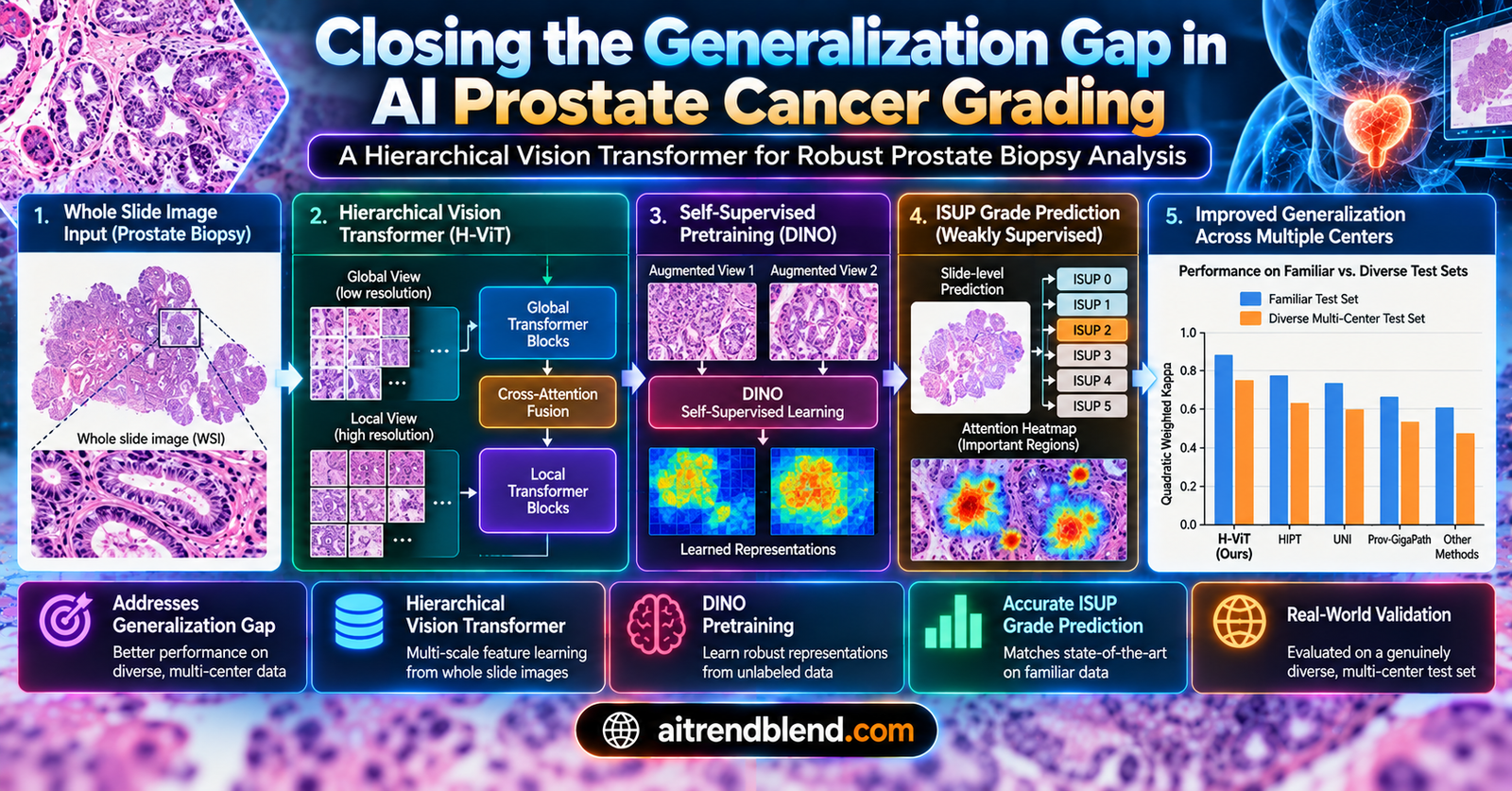
- The researchers built and rigorously tested Hierarchical Vision Transformers, a three-stage architecture that reads a prostate biopsy at cell, tissue region, and whole slide scale, for grading prostate cancer severity.
- Their best model matched the top algorithms from the PANDA computational pathology challenge on familiar, same-center test data, reaching a quadratic weighted kappa of 0.916, and outperformed all of them on a genuinely diverse, seven-center dataset built specifically to stress test generalization.
- Pretraining the model exclusively on prostate tissue beat pretraining on a much larger, general-purpose, multi-organ pathology foundation model, a result the authors tie to that larger model overfitting to center-specific visual signatures rather than learning universal features.
- A version of the architecture that lets gradients flow through more of the network, called Local H-ViT, beat the more parameter-efficient frozen version at every single configuration tested, a result that runs counter to the original architecture’s own published guidance.
- The authors state plainly that their model is intended as a decision-support tool for pathologists who already have established workflows, not a standalone diagnostic system, and this article treats that framing as authoritative.
A biopsy slide too big for a computer to look at all at once
Prostate cancer is, by the paper’s own framing, the second most frequently diagnosed cancer and the fifth leading cause of cancer death among men worldwide. Grading how aggressive a tumor looks under the microscope, a task pathologists perform using a system called Gleason patterns rolled up into International Society of Urological Pathology, or ISUP, grade groups, directly shapes what happens next for a patient, anywhere from watchful waiting to surgery. As caseloads climb, so does the appeal of a computational second opinion.
The technical obstacle is almost comically literal. A digitized whole slide image, the standard format pathology AI works with, can run to billions of pixels, far beyond what a conventional GPU can hold in memory at once. The field’s answer has generally been to break a slide into smaller patches and train on those instead, often under a weakly supervised paradigm called Multiple Instance Learning, where the model only ever sees a single label for the entire slide rather than pixel-level annotations for every patch, since asking pathologists to trace every tumor boundary by hand is, as the authors put it, labor intensive and sometimes impractical.
The catch with ordinary patch-based methods is that they treat each small patch mostly in isolation, missing the broader spatial context of how tissue is organized across the slide. Hierarchical Vision Transformers, first introduced for computational pathology by Chen and colleagues in 2022 under the name HIPT, were built specifically to close that gap, borrowing an idea from how Transformers were adapted to handle long text documents and applying the same multi-scale trick to gigapixel images.
Why the original architecture needed a harder test
HIPT’s original evaluation focused on cancer subtyping and survival prediction, tasks the authors of this new paper argue are meaningfully simpler than prostate grading, and it was never independently tested outside its original authors’ own experiments. That gap in independent validation is exactly what this paper sets out to close, examining four separate design choices, self-supervised pretraining strategy, which of two architectural variants to use, how much spatial context to feed the model, and which loss function best suits an ordinal grading scale, then testing the resulting best configuration against genuinely unfamiliar clinical data.
How a three-stage transformer reads a slide it cannot see all at once
The architecture works by nesting three separate Vision Transformers, each responsible for a different physical scale of the tissue. A patch-level Transformer breaks 256 by 256 pixel patches into 16 by 16 pixel tokens, capturing cell-to-cell interactions. Its output feeds a region-level Transformer, which aggregates non-overlapping 256 by 256 patches within a larger 4096 by 4096 pixel region, building context-aware embeddings that span clusters of cells. Finally, a slide-level Transformer pools every region-level embedding from across the whole slide into a single representation, which gets projected to the class logits used for the final grading prediction.
Two variants of this stack were tested side by side. Global H-ViT, which replicates the original HIPT’s best configuration, keeps both the patch-level and region-level Transformers frozen after pretraining, training only the slide-level Transformer on the actual grading task, resulting in roughly 0.6 million trainable parameters. Local H-ViT keeps only the patch-level Transformer frozen, allowing gradients to flow through both the region-level and slide-level Transformers during training, at the cost of a larger 3.5 million trainable parameters and considerably heavier compute.
Teaching the first two layers to see tissue before ever showing them a grade
Both the patch-level and region-level Transformers are pretrained without any grading labels at all, using a self-supervised technique called DINO, where a student network is trained to match the output of a slower-moving teacher network on different augmented views of the same input image.
The student network, parameterized by \( \theta_s \), is trained to minimize cross entropy \( H(a,b) = -a \log b \) between the teacher’s output probability distribution \( p_t \) on a global view and the student’s output distribution \( p_s \) on other views, including smaller local crops the teacher never sees. This forces the student to learn representations that generalize from a partial, zoomed-in view of tissue to the fuller picture.
The patch-level Transformer, a ViT-Small with 22 million parameters, was pretrained on roughly 2.4 million non-overlapping 256 by 256 patches extracted from training slides, for 50 epochs, taking 3 days across 4 GeForce RTX 3080 Ti GPUs. To monitor this unsupervised process, the authors built a small side benchmark, a balanced set of 5,000 benign and 5,000 tumor patches drawn from a subset of slides with pixel-level annotations, and tracked how well a simple k-nearest neighbor classifier built on the evolving features could separate the two classes, entirely independent of the actual grading task the model would eventually be trained for.
The choice that mattered more than the architecture, pretraining domain
The paper’s clearest and most consequential finding concerns what data the first two Transformers see before grading ever enters the picture. The original HIPT weights were pretrained on 10,678 slides from The Cancer Genome Atlas, spanning 33 different cancer types, but only 4 percent of those slides were prostate resections. Applying those TCGA-pretrained weights directly to prostate grading in this paper’s PANDA setup produced quadratic weighted kappa scores as low as 0.42 on the public test set.
Retraining the same architecture using self-supervised pretraining exclusively on prostate biopsies from the PANDA dataset itself, rather than the broad multi-organ TCGA collection, produced a dramatic jump.
| Region size and pretraining source | Global H-ViT, test kappa | Local H-ViT, test kappa |
|---|---|---|
| 4096 pixel regions, TCGA pretrained | 0.422 | 0.761 |
| 4096 pixel regions, PANDA pretrained | 0.721 | 0.882 |
| 1024 pixel regions, TCGA pretrained | 0.599 | 0.774 |
| 1024 pixel regions, PANDA pretrained | 0.844 | 0.878 |
The gain from switching pretraining data was far larger for Global H-ViT, averaging a 68 percent improvement, than for Local H-ViT, which averaged a 14 percent improvement. The explanation the authors offer is architectural rather than mysterious, Global H-ViT keeps its first two Transformers completely frozen, so if their pretrained features are a poor fit for prostate tissue, nothing downstream can compensate. Local H-ViT allows gradients to flow through the region-level Transformer during the actual grading task, giving it room to partially correct for suboptimal pretraining even when starting from the weaker TCGA weights.
A bigger foundation model is not automatically a better one
The authors pushed this question further by testing UNI, a considerably larger ViT-Large foundation model pretrained on more than 100,000 hematoxylin and eosin stained slides spanning a wide range of tissue types and diseases, described as one of the leading publicly available foundation models in histopathology. On the PANDA test sets specifically, UNI performed comparably to the smaller, prostate-specific ViT-Small the authors had pretrained themselves. The story changed sharply once the model faced genuinely unfamiliar clinical data, a result covered in detail below, and the authors connect this directly to separate published research finding that pathology foundation models tend to learn center-specific representations rather than truly universal ones.
Context size, loss function, and an architectural surprise
Beyond pretraining, the researchers systematically varied how much spatial context the model sees at once, testing 4096, 2048, and 1024 pixel square regions, and which loss function best captures the fact that ISUP grades are ordered, not simply five unrelated categories. Standard cross entropy, which treats a one-grade error the same as a four-grade error, sat at the bottom of the five options tested, alongside two more sophisticated rank-consistent methods called CORAL and CORN, and an ordinal variant of cross entropy. Reframing the entire task as regression and training with mean squared error, which naturally respects the ordering of grades, produced the best quadratic weighted kappa scores for both architectural variants.
On context size, the authors found something specific to this task rather than a universal rule, that prostate grading signal tends to live within a scale smaller than the field’s original default. Since Gleason growth patterns, the microscopic feature pathologists actually grade on, typically fit within a 1024 by 1024 pixel window at the resolution used here, feeding the model unnecessarily large 4096 pixel regions diluted the signal with more background tissue and offered no benefit, while smaller regions produced a finer, less noisy tiling of the slide.
The clearest departure from the original HIPT design came from comparing Global and Local H-ViT directly. Local H-ViT, the more computationally expensive, gradient-unlocked variant, outperformed Global H-ViT across every single configuration of pretraining source, region size, and loss function tested, a result the authors note explicitly deviates from the conclusions of the architecture’s original creators, who favored the frozen approach. To confirm this was not an artifact specific to prostate grading, they replicated a breast cancer subtyping experiment from the original HIPT paper and found the same pattern held, Local H-ViT’s own reimplementation reached an AUC of 0.894 against the original paper’s reported 0.827 for the same architecture.
The dataset, and the quiet data leakage problem the authors found and fixed
Model development ran on PANDA, the Prostate cANcer graDe Assessment dataset, described as the largest publicly available collection of hematoxylin and eosin stained prostate whole slide images, with 11,554 biopsies sourced from Radboud University Medical Center in the Netherlands and Karolinska Institutet in Sweden. Reference grades for the Radboud portion came from routine clinical pathology reports, while the Karolinska development portion was labeled by a single uropathologist following routine workflow. The held-out test sets used tighter consensus standards, a panel of three expert uropathologists for the Radboud test cases and four for the Karolinska test cases.
Before training, the authors uncovered and addressed a subtle bias problem the original PANDA challenge organizers themselves had flagged, that many slides in the dataset are serial sections cut from the same underlying tissue block, meaning near-duplicate images can end up split across training and internal tuning sets, quietly inflating a model’s apparent performance during development. Since PANDA provides no direct mapping from slide to originating tissue block, the authors built one themselves using image hashing, identifying 297 clusters of visually near-identical slides covering roughly 6 percent of the development set, then made sure slides from the same cluster always stayed together in the same data split. A second cleanup step addressed ordinary label noise from the manual grading process, training an initial model, measuring the gap between its soft predictions and the recorded ground truth for every slide, and discarding the 10 percent of slides with the largest such gap before finalizing the training splits used for every subsequent experiment.
What actually happened on unfamiliar data
The paper’s central claim rests on comparing performance across three settings of increasing difficulty, the official PANDA test sets, which despite being held out still draw from the same two source centers as training, a private external dataset from Karolinska University Hospital deliberately curated to span a wide range of grades, and a crowd-sourced dataset assembled by a separate research group specifically to stress test generalization across genuinely different institutions.
| Test setting | Best competing PANDA team | The paper’s best model | Statistically significant difference |
|---|---|---|---|
| PANDA combined public and private test set | 0.928 (Save The Prostate) | 0.916 | No, p = 0.1235 |
| Karolinska University Hospital external set | 0.899 (NS Pathology) | 0.895 | No, p = 0.9333 |
| Crowd-sourced, seven-center diverse set | 0.862 (PND) | 0.877, the highest score of any model tested | No, p = 0.7313 |
Read that table carefully, because the honest version of this story is more nuanced than a simple win. On the two settings closest to the original training data, the paper’s model was statistically indistinguishable from the best-performing competing team, meaning it matched, rather than beat, the state of the art. On the hardest, most diverse dataset, drawn from seven different centers across multiple countries and including staining protocols entirely absent from the PANDA training data, the paper’s model posted the single highest quadratic weighted kappa of any method evaluated, 0.877 against the next best team’s 0.862. But by the authors’ own statistical test, even that numerically largest gap did not reach significance against the second place team. The honest summary is that this model was the best performer on the hardest test by a real margin, while also being one where the authors’ own significance testing could not rule out that some of that gap reflects chance rather than a guaranteed, repeatable advantage.
Notably, our best model matched state-of-the-art algorithms on in-domain data while consistently outperforming them on out-domain data. This result sets a new benchmark in prostate biopsy cancer grading, narrowing the generalization gap. From the paper’s discussion section, summarizing its central claim
The gap between the two external test sets is itself informative. Performance on the Karolinska University Hospital dataset stayed high across nearly every model the authors compared against, which they attribute to that dataset’s visual similarity to the Karolinska-sourced portion of the PANDA training data. Performance on the crowd-sourced dataset told a very different story. Several PANDA challenge participants’ models, which had performed competitively on the official test sets, showed sharp drops on this genuinely unfamiliar data, underscoring that a model’s showing on a same-source held-out test set can be a poor guide to how it behaves in a truly different clinical environment.
The UNI-based version of the model, which had performed comparably to the prostate-specific version on PANDA’s own test sets, showed a much steeper decline once tested on the two external cohorts, dropping to 0.867 on the Karolinska external set and 0.793 on the crowd-sourced set, compared to 0.895 and 0.877 for the prostate-specific model. The authors interpret this as evidence that even a very large, broadly trained pathology foundation model can end up learning features tied to the specific centers and scanners represented in its own training data, rather than features that transfer cleanly to new ones.
Making the model’s attention interpretable, and honest about its limits
A separate contribution addresses a practical concern for any clinician asked to trust a model’s output, understanding which parts of a slide actually drove a given prediction. The original HIPT paper visualized attention only from its two frozen, pretrained Transformers, meaning the resulting heatmaps could only ever show generic, task-agnostic visual features learned before the model ever saw a single grading label, offering little insight into what specifically drove the final prediction.
This paper introduces a tunable parameter, gamma, that blends attention scores from the frozen, pretraining-derived Transformers with attention from the Transformers actually trained on the grading task itself.
For a given pixel location, the factorized attention score blends the individual attention contributions \( a^i_{(x,y)} \) from each of the \( N \) Transformers, weighted by \( \gamma \in [0,1] \) and whether that Transformer, \( T_i \), was frozen during training, indicated by \( \mathbb{1}_F(T_i) \), with \( \beta \) a normalizing constant. Setting \( \gamma \) near zero emphasizes features learned purely during self-supervised pretraining, while setting it above 0.5 shifts emphasis toward features the model actually learned while training on real grading labels.
Because the biological signal pathologists actually use for grading, the architecture of glandular tissue, lives at a coarser scale than the cell-level detail the frozen patch-level Transformer captures, the authors recommend setting gamma above 0.5 in practice, favoring the coarser, task-specific attention over the finer, task-agnostic kind. This is a genuinely more informative visualization than the original method, but the authors are careful not to oversell it, stating directly that heatmaps alone do not fully explain how a highlighted region relates to a specific predicted grade, and that pathologists may reasonably remain cautious about adopting a tool whose reasoning process is not fully transparent.
Clinical translation gap
The authors position their own work with unusual directness on this point, and it is worth quoting rather than softening. They state that their model would best serve as a decision-support tool rather than a standalone diagnostic system, adding an extra layer of confidence for pathologists who already have established workflows, not replacing the pathologist’s own judgment. That framing matters because every result in this paper measures agreement with expert human grading on retrospective, already-diagnosed cases, not real-time clinical performance, patient outcomes, or how the tool would behave integrated into an actual pathology workflow where a clinician interacts with its output under time pressure.
The generalization testing in this paper, while considerably more rigorous than typical same-center validation, still covers a specific and limited slice of the real world, biopsies from institutions in the Netherlands, Sweden, France, Portugal, and Turkey, scanned on a handful of specific scanner models. A genuinely global deployment would encounter staining protocols, scanner hardware, tissue processing conventions, and patient populations well beyond even this diverse test set. The paper’s own ethics statement confirms this is a retrospective study using existing, de-identified biopsy data, with an ethical committee waiving the need for new patient consent, not a prospective clinical trial evaluating the tool’s effect on real diagnostic decisions or patient outcomes.
Honest limitations
Several boundaries deserve to be named plainly, using only what the paper itself reports. The headline generalization win on the crowd-sourced dataset, while numerically the best score of any method tested, was not statistically significant against the second-best team by the authors’ own permutation test, a distinction easy to lose in any summary that leads only with the raw numbers. On the two other, less diverse test settings, the model matched rather than exceeded the best competing methods.
The augmentation strategy used throughout training has a specific, acknowledged gap, the authors applied augmentation only during the self-supervised pretraining stage, using DINO’s default settings originally designed for natural photographs rather than pathology images, and applied no augmentation at all during the actual weakly supervised grading training, because augmenting pixel data at that stage would require re-embedding every augmented region independently, an expense the authors flag as a reason for future work on cheaper, feature-space augmentation instead. The interpretability method, while an improvement over prior work, still cannot fully explain how a highlighted region relates to a specific predicted grade, a limitation the authors state directly rather than leaving implicit.
Finally, several of the paper’s authors disclose financial relationships with companies operating in digital pathology and medical imaging, including equity or consulting ties to Aiosyn BV, Clinsight AB, Canon Health Informatics, Philips, ContextVision, and Sectra, alongside various research foundation funding. Such disclosures are standard practice and do not by themselves undermine a paper’s findings, particularly given the paper’s own restrained framing of its results and its direct statement that this system is meant as decision support rather than autonomous diagnosis, but they are worth surfacing plainly for anyone weighing how much independent commercial interest might intersect with this specific line of research.
Where this points next
The authors name two concrete directions themselves. Cheaper, feature-space data augmentation during the actual grading training phase, rather than only during self-supervised pretraining, is flagged as an open opportunity to potentially improve performance further without the computational cost of re-embedding augmented pixel regions. On interpretability, they propose deriving label-specific attention scores that would let a pathologist directly query which parts of an image the model associates with a particular grade, a more targeted and clinically legible explanation than a single blended heatmap can currently offer.
Conclusion
What makes this paper worth reading past its headline kappa score is the discipline of its own comparisons. Rather than reporting a single strong number on a single familiar test set, the authors built two genuinely different, increasingly demanding external evaluations and reported exactly where their model matched the competition, where it numerically led, and where that lead did not clear the bar of statistical significance. That is a more useful, and more trustworthy, way to report a generalization claim than simply asserting one.
The pretraining result deserves to travel further than this specific paper. A smaller model trained exclusively on the tissue type it will actually be used on beat a substantially larger, more broadly trained foundation model exactly where it mattered most, on data from institutions the model had never encountered during training. That is a genuinely useful, and somewhat counterintuitive, data point for a research community currently investing heavily in ever larger, ever more general pathology foundation models, a reminder that scale and generality are not automatically the same thing as robustness.
The architectural finding, that letting more of the network adapt to the actual task consistently beat the more conservative, frozen approach recommended by the original architecture’s own authors, is a useful corrective too, though the paper is careful to frame it as conditional rather than universal, a recommendation that depends on having enough labeled data to support the larger model’s greater capacity, not a blanket claim that more trainable parameters is always the better choice.
None of this closes the distance between a strong benchmark result and a tool a pathologist would actually rely on day to day. The authors say so themselves, describing their system as an additional layer of confidence for a pathologist’s existing workflow rather than a replacement for one, and naming directly the interpretability gaps and augmentation limitations still standing between this result and that kind of practical integration. What the paper demonstrates convincingly, within that honestly stated scope, is that a hierarchical, multi-scale reading of a gigapixel biopsy slide, built on pretraining data that actually matches the tissue being examined, is a genuinely more robust approach to a hard clinical grading problem than either a narrower patch-based method or a bigger, more generic foundation model managed to be on the same test.
For a field where a model’s real value only shows up once it leaves the hospital that trained it, a paper willing to report a numerically winning result alongside the statistical test that keeps it honest is doing something more useful than chasing one more decimal point on a familiar leaderboard.
Reference implementation of the core architecture in PyTorch
The following is an original, simplified, runnable PyTorch implementation inspired by the three-stage hierarchical Transformer, the factorized attention blending mechanism, and the ordinal regression loss described in the paper. It is a compact educational reconstruction of the core architecture, not the authors’ own code, built to illustrate the approach on dummy data with a working smoke test.
# hvit_prostate_grading_core.py
# Educational reimplementation of the three-stage Hierarchical Vision
# Transformer, the factorized attention blending mechanism, and the
# MSE-based ordinal grading loss, inspired by "Hierarchical Vision
# Transformers for prostate biopsy grading: Towards bridging the
# generalization gap", Medical Image Analysis, 2025.

import torch
import torch.nn as nn
import torch.nn.functional as F

NUM_GRADES = 5  # ISUP grade groups 0 through 4
PATCH_TOKEN_DIM = 192
REGION_EMBED_DIM = 192


class SimpleTransformerBlock(nn.Module):
    """A single self-attention block standing in for one stage of the
    hierarchy. Returns both the pooled output and the raw attention
    weights, which the factorized attention mechanism later blends."""
    def __init__(self, dim, num_heads=4):
        super().__init__()
        self.attn = nn.MultiheadAttention(dim, num_heads, batch_first=True)
        self.norm = nn.LayerNorm(dim)
        self.cls_token = nn.Parameter(torch.zeros(1, 1, dim))

    def forward(self, tokens):
        batch = tokens.shape[0]
        cls = self.cls_token.expand(batch, -1, -1)
        sequence = torch.cat([cls, tokens], dim=1)
        attended, attn_weights = self.attn(sequence, sequence, sequence, need_weights=True)
        pooled = self.norm(attended[:, 0])  # the CLS token summarizes this level
        # attention from the CLS token onto every other token, used for heatmaps
        cls_attention = attn_weights[:, 0, 1:]
        return pooled, cls_attention


class HierarchicalViT(nn.Module):
    """A compact three-stage stand in for the patch-level, region-level,
    and slide-level Transformers described in Section 3.1. The frozen
    flag on each stage mirrors the Global versus Local H-ViT distinction."""
    def __init__(self, freeze_patch=True, freeze_region=True):
        super().__init__()
        self.patch_encoder = nn.Linear(768, PATCH_TOKEN_DIM)  # stand in for a pretrained patch CNN embedding
        self.patch_transformer = SimpleTransformerBlock(PATCH_TOKEN_DIM)
        self.region_transformer = SimpleTransformerBlock(REGION_EMBED_DIM)
        self.slide_transformer = SimpleTransformerBlock(REGION_EMBED_DIM)
        self.grade_head = nn.Linear(REGION_EMBED_DIM, 1)  # regression head, per the MSE loss finding

        self.freeze_patch = freeze_patch
        self.freeze_region = freeze_region
        if freeze_patch:
            for p in self.patch_transformer.parameters():
                p.requires_grad = False
        if freeze_region:
            for p in self.region_transformer.parameters():
                p.requires_grad = False

    def forward(self, raw_patch_tokens, patches_per_region, regions_per_slide):
        """raw_patch_tokens: (batch, regions_per_slide, patches_per_region, 768)
        a stand in for pretrained low-level patch features."""
        batch = raw_patch_tokens.shape[0]
        embedded = self.patch_encoder(raw_patch_tokens)
        embedded = embedded.reshape(batch * regions_per_slide, patches_per_region, PATCH_TOKEN_DIM)

        region_embeds, patch_attn = self.patch_transformer(embedded)
        region_embeds = region_embeds.reshape(batch, regions_per_slide, REGION_EMBED_DIM)

        slide_embed_input, region_attn = self.region_transformer(region_embeds)
        slide_embed_input = slide_embed_input.unsqueeze(1).expand(-1, regions_per_slide, -1)

        slide_repr, slide_attn = self.slide_transformer(region_embeds)
        grade_pred = self.grade_head(slide_repr).squeeze(-1)

        attentions = {"patch": patch_attn, "region": region_attn, "slide": slide_attn}
        return grade_pred, attentions


def factorized_attention(attentions, frozen_flags, gamma):
    """Implements Eq. 2, blending attention from frozen (task-agnostic)
    and trained (task-specific) transformers according to gamma."""
    stages = list(attentions.keys())
    n = len(stages)
    n_frozen = sum(1 for s in stages if frozen_flags[s])
    beta = (n - n_frozen) * gamma + n_frozen * (1 - gamma)

    total = 0.0
    for stage in stages:
        weight = (1 - gamma) if frozen_flags[stage] else gamma
        # mean over the attention map's own dimension to get one score per region, for illustration
        stage_score = attentions[stage].mean(dim=-1) if attentions[stage].dim() > 1 else attentions[stage]
        total = total + weight * stage_score.mean()
    return total / (beta + 1e-8)


def ordinal_grading_loss(predicted_grade, true_grade):
    """Implements the MSE regression loss the paper found superior to
    plain cross entropy, ordinal CE, CORAL, and CORN for ISUP grading."""
    return F.mse_loss(predicted_grade, true_grade.float())


def quadratic_weighted_kappa(preds, targets, num_classes=NUM_GRADES):
    """A minimal reference implementation of Cohen's quadratic weighted
    kappa, the paper's primary evaluation metric, for rounded predictions."""
    preds = preds.round().clamp(0, num_classes - 1).long()
    targets = targets.long()
    confusion = torch.zeros(num_classes, num_classes)
    for p, t in zip(preds.tolist(), targets.tolist()):
        confusion[t, p] += 1

    weights = torch.zeros(num_classes, num_classes)
    for i in range(num_classes):
        for j in range(num_classes):
            weights[i, j] = ((i - j) ** 2) / ((num_classes - 1) ** 2)

    row_sums = confusion.sum(dim=1, keepdim=True)
    col_sums = confusion.sum(dim=0, keepdim=True)
    expected = row_sums @ col_sums / confusion.sum()

    observed_disagreement = (weights * confusion).sum()
    expected_disagreement = (weights * expected).sum()
    if expected_disagreement == 0:
        return torch.tensor(1.0)
    return 1.0 - observed_disagreement / expected_disagreement


def smoke_test():
    """Runs one forward and backward pass on random dummy data to confirm
    every module is wired together correctly, using Local H-ViT style
    settings where only the patch-level stage stays frozen."""
    torch.manual_seed(0)
    model = HierarchicalViT(freeze_patch=True, freeze_region=False)
    optimizer = torch.optim.Adam(filter(lambda p: p.requires_grad, model.parameters()), lr=2e-4)

    batch, regions_per_slide, patches_per_region = 2, 6, 16
    dummy_patches = torch.randn(batch, regions_per_slide, patches_per_region, 768)
    dummy_grades = torch.randint(0, NUM_GRADES, (batch,))

    predicted_grade, attentions = model(dummy_patches, patches_per_region, regions_per_slide)
    loss = ordinal_grading_loss(predicted_grade, dummy_grades)

    optimizer.zero_grad()
    loss.backward()
    optimizer.step()

    frozen_flags = {"patch": True, "region": False, "slide": False}
    factorized_score = factorized_attention(attentions, frozen_flags, gamma=0.7)
    kappa = quadratic_weighted_kappa(predicted_grade.detach(), dummy_grades)

    print("Predicted grades", predicted_grade.detach().tolist())
    print("Training loss", float(loss))
    print("Factorized attention score at gamma=0.7", float(factorized_score))
    print("Quadratic weighted kappa on this random batch", float(kappa))
    print("Smoke test completed without errors")


if __name__ == "__main__":
    smoke_test()
Frequently asked questions
What is prostate cancer grading and why does an AI system need to be involved
Prostate cancer grading is the process by which pathologists examine biopsy tissue under a microscope and assign an ISUP grade group based on how aggressive the cancer’s growth patterns look, a grade that directly informs treatment decisions ranging from active surveillance to surgery. This paper explores whether a computational model can perform this grading task with accuracy comparable to expert pathologists, motivated by rising patient caseloads placing increasing pressure on pathology departments.
What is a Hierarchical Vision Transformer and why does it matter for this task
A Hierarchical Vision Transformer processes an image at multiple nested scales using separate Transformer networks, one for small cell-level patches, one for larger tissue regions, and one for the whole slide. This design exists specifically because a full pathology slide can contain billions of pixels, far too many for a single neural network to process directly, so the hierarchy lets the model build up a whole-slide understanding from smaller, manageable pieces.
Does this model diagnose prostate cancer on its own
No. The authors state directly that their model is intended to serve as a decision-support tool that adds an extra layer of confidence for pathologists who already have established diagnostic workflows, not a standalone diagnostic system. Every result in the paper measures how closely the model’s grading matches expert pathologists on already-collected biopsy images with known outcomes, not real-time clinical decision making.
Did the model actually outperform existing methods
The results are more nuanced than a simple win. On the official PANDA challenge test sets and a first external Karolinska Hospital dataset, the model statistically matched, but did not significantly exceed, the best competing methods. On a harder, more diverse seven-center crowd-sourced dataset, the model achieved the single highest score of any method tested, but the authors’ own statistical test found that this specific gap over the second-best competing team was not statistically significant.
Why did a smaller, prostate-specific model outperform a much larger general pathology foundation model
On the paper’s own in-domain PANDA test sets, the smaller prostate-specific model and the larger multi-organ foundation model called UNI performed comparably. The gap opened up specifically on the two external, out-of-domain test sets, where the larger foundation model’s performance dropped more sharply. The authors attribute this to the foundation model potentially learning representations tied to the specific centers and scanners in its own training data, rather than features that transfer as cleanly to genuinely new clinical settings.
What did the researchers find about the model’s internal attention or explainability
The researchers introduced a tunable method for blending attention scores from the model’s pretrained, frozen layers with attention from the layers actually trained on the grading task, producing more clinically relevant heatmaps than prior work. However, the authors state directly that these heatmaps alone do not fully explain how a highlighted region relates to a specific predicted grade, and that further work on more targeted, label-specific explanations is still needed before pathologists could be expected to fully trust the model’s reasoning.
Read the original research
This analysis is based on the peer reviewed, open access paper published in Medical Image Analysis, volume 105, 2025.
Pingback: 7 Astonishing Ways DIOR-ViT Transforms Cancer Grading (Avoiding Common Pitfalls) - aitrendblend.com
Pingback: 7 Unbelievable Wins & Pitfalls of Context-Aware Knowledge Distillation for Disease Prediction - aitrendblend.com
Pingback: 9 Explosive Strategies & Hidden Pitfalls in Data-Centric Directed Graph Learning - aitrendblend.com
Pingback: 5 Revolutionary Advancements in Medical Image Segmentation: How SDCL Outperforms Existing Methods (With Math Explained) - aitrendblend.com
Pingback: Bidirectional Copy-Paste Revolutionizes Semi-Supervised Medical Image Segmentation (21% Dice Improvement Achieved, but Challenges Remain) - aitrendblend.com
Pingback: 7 Powerful Problems and Solutions: Overcoming and Transforming Long-Tailed Semi-Supervised Learning with FlexDA & ADELLO - aitrendblend.com
Pingback: GenSeg: Revolutionizing Medical Image Segmentation with End-to-End Synthetic Data Generation (2025 Breakthrough) - aitrendblend.com
Pingback: 5 Revolutionary Breakthroughs in AI-Powered Cardiac Ultrasound: Unlocking Self-Supervised Learning (While Overcoming Manual Labeling Challenges) - aitrendblend.com
Pingback: 6 Groundbreaking Innovations in Diabetic Retinopathy Detection: A 2025 Breakthrough - aitrendblend.com
Pingback: 6 Groundbreaking Hybrid Features for Breast Cancer Classification: Power of AI & Machine Learning - aitrendblend.com
Pingback: 5 Revolutionary Insights from biM-CGN: Boosting Recommendation Accuracy and Diversity - aitrendblend.com
Pingback: 7 Powerful Reasons BAST-Mamba Is Revolutionizing Binaural Sound Localization — Despite the Challenges - aitrendblend.com
Pingback: 7 Revolutionary Advancements in Functional Data Clustering with Fdmclust (And What's Holding It Back) - aitrendblend.com
Pingback: Revolutionizing Lower Limb Motor Imagery Classification: A 3D-Attention MSC-T3AM Transformer Model with Knowledge Distillation - aitrendblend.com
Pingback: 7 Revolutionary Ways Event-Based Action Recognition is Changing AI (And Why It’s Not Perfect Yet) - aitrendblend.com
Pingback: 7 Powerful Insights from a Groundbreaking Study on Motion Processing and Neural Adaptation - aitrendblend.com
Pingback: 7 Groundbreaking Innovations in Deep Bi-Directional Predictive Coding (DBPC): The Future of Efficient Neural Networks - aitrendblend.com
Pingback: 7 Revolutionary Ways to Compress BERT Models Without Losing Accuracy (With Math Behind It) - aitrendblend.com
Pingback: 7 Breakthroughs: How Uncertainty-Guided AI is Revolutionizing Malaria Detection in Blood Smears (Life-Saving AI vs. Deadly Parasites!) - aitrendblend.com
Pingback: Decoding Olfactory Response with TACAF: A Breakthrough in EEG and Breathing Signal Fusion - aitrendblend.com
Pingback: UNETR++ vs. Traditional Methods: A 3D Medical Image Segmentation Breakthrough with 71% Efficiency Boost - aitrendblend.com
Pingback: EFAM-Net: The Future of Skin Lesion Classification with Enhanced Feature Fusion (2024 Breakthrough) - aitrendblend.com
Pingback: 10 Groundbreaking Innovations in Treatment-Aware Diffusion Models for Longitudinal MRI and Diffuse Glioma - aitrendblend.com
Pingback: DeepMetaForge: Revolutionizing Skin Lesion Classification with Vision-Transformers and Metadata Fusion (2023 Study) - aitrendblend.com
Pingback: 10X Faster Retinal Vessel Segmentation: How MaskVSC Eliminates Fragmentation for Superior Accuracy - aitrendblend.com
Pingback: 7 Revolutionary Graph-Transformer Breakthrough: Why This AI Model Outperforms (And What It Means for Cancer Diagnosis) - aitrendblend.com
Pingback: 7 Revolutionary Breakthroughs in Cancer Survival Prediction (And 1 Critical Flaw You Can’t Ignore) - aitrendblend.com
Pingback: 7 Revolutionary Ways ConvexAdam Beats Traditional Methods (And Why Most Fail) - aitrendblend.com
Pingback: 7 Revolutionary Breakthroughs and 1 Major Challenge in Nanoscale Biosensing Using AI-Driven Capacitance Spectroscopy - aitrendblend.com
Pingback: Revolutionary Breakthroughs in Time Series Anomaly Detection — The MAAT Model That Outperforms (and 1 Fatal Flaw) - aitrendblend.com
Pingback: 11 Breakthrough Deep Learning Tricks That Eliminate Finger-Vein Recognition Failures for Good - aitrendblend.com
Pingback: 7 Revolutionary Breakthroughs in Skin Cancer Detection: How a New AI Model Outperforms Experts (And Why Older Methods Fail) - aitrendblend.com
Pingback: 7 Shocking Ways Merging Korean Language Models Boosts LLM Reasoning (And 1 Dangerous Pitfall to Avoid) - aitrendblend.com
Pingback: 7 Revolutionary Breakthroughs in Diabetes Tech (Why Most Fail & How This AI Model Succeeds) - aitrendblend.com
Pingback: 5 Shocking Secrets of Skin Cancer Detection: How This SSD-KD AI Method Beats the Competition (And Why Others Fail) - aitrendblend.com
Pingback: 7 Revolutionary Breakthroughs in HDR Video (and the 1 Fatal Flaw Holding It Back) - aitrendblend.com
Pingback: 7 Revolutionary Breakthroughs in MR Spectroscopic Imaging: How a Powerful New Method Beats Old, Inaccurate Techniques - aitrendblend.com
Pingback: 7 Revolutionary Breakthroughs in MRI Super-Resolution – The Good, the Bad, and the Future of HFMT - aitrendblend.com
Pingback: 7 Revolutionary Breakthroughs in Hollow Sphere Simulation: How IGA Outperforms Traditional FEA (And When It Fails) - aitrendblend.com
Pingback: 7 Revolutionary Wins & Costly Mistakes in Structural Optimization: How ASM-Powered Chaos Game Optimization (CGO) Outperforms Old Methods - aitrendblend.com
Pingback: 7 Revolutionary Breakthroughs in Skin Lesion Segmentation — The Dark Truth About Traditional Methods vs. ESC-UNET’s AI Power - aitrendblend.com
Pingback: 7 Revolutionary Breakthroughs in Diabetic Retinopathy Detection – How AI Is Saving Sight (And Why Most Mobile Apps Fail) - aitrendblend.com
Pingback: Revolutionary Breakthroughs in Breast Cancer Detection: The +95% Accuracy Model vs. Outdated Methods - aitrendblend.com
Pingback: 9 Revolutionary ETDHDNet Breakthrough: The Ultimate AI Tool That’s Transforming Tuberculosis Detection (And Why Older Methods Are Failing) - aitrendblend.com
Pingback: Shocking Failures of Standard AI Models (And the 1 Solution That Fixes Them All) – AdaPAC Explained - aitrendblend.com
Pingback: 7 Revolutionary Breakthroughs in Continual Learning: The Rise of Adapt&Align - aitrendblend.com
Pingback: 7 Shocking Truths About Wearable AI in Healthcare: The Good, The Bad, and The Overhyped - aitrendblend.com
Pingback: 7 Revolutionary Breakthroughs in AI Uncertainty Estimation: The Good, the Bad, and the Future of Trustworthy AI - aitrendblend.com
Pingback: 7 Revolutionary Breakthroughs in Cancer Immunotherapy: How AI is Transforming ICD Screening - aitrendblend.com
Pingback: 7 Revolutionary Breakthroughs in Thyroid Cancer AI: How DualSwinUnet++ Outperforms Old Models - aitrendblend.com
Pingback: 7 Revolutionary Breakthroughs in Cardiac Motion Analysis: How a New AI Model Outperforms Old Methods (And Why It Matters) - aitrendblend.com
Pingback: 7 Revolutionary Breakthroughs in NPH Diagnosis: the Future of AI-Powered Brain Scans - aitrendblend.com
Pingback: 7 Revolutionary Breakthroughs in Bacteria Detection: How EmiNet Outperforms Old Methods - aitrendblend.com
Pingback: 3 Revolutionary FCS-MPDTC Breakthroughs That Slash Energy Waste in Linear Motors - aitrendblend.com
Pingback: Revolutionary Ways to Boost Compressor Efficiency by 3.2% - aitrendblend.com
Pingback: Revolutionary Breakthroughs in Skin Cancer Detection: ConvNeXtV2 & Focal Attention - aitrendblend.com
Pingback: 7 Shocking Mistakes in Knowledge Distillation (And the 1 Breakthrough Fix That Changes Everything) - aitrendblend.com
Pingback: 7 Revolutionary Breakthroughs in AI Disease Grading — The Good, the Bad, and the Future of UMKD - aitrendblend.com
Pingback: 7 Shocking Breakthroughs in Spiking Neural Networks: How HTA-KL Crushes Accuracy & Efficiency - aitrendblend.com
Pingback: 7 Revolutionary Breakthroughs in Knowledge Distillation: Why Swapped Logit Distillation Outperforms Old Methods - aitrendblend.com
Pingback: 7 Revolutionary Breakthroughs in Endometriosis Detection: How AI is Transforming Diagnosis - aitrendblend.com
Pingback: 7 Shocking Ways AI Fails at Medical Diagnosis (And the Brilliant Fix That Saves Lives) - aitrendblend.com
Pingback: 7 Revolutionary Breakthroughs in Gene Network Mapping - aitrendblend.com
Pingback: 7 Breakthrough AI Insights: How Machine Learning Predicts Glioma Grading - aitrendblend.com
Pingback: Revolutionary Breakthroughs in 3D Organ Detection: How Organ-DETR Outperforms Old Methods (+10.6 mAP Gain!) - aitrendblend.com
Pingback: 7 Revolutionary VibNet Breakthrough Detects Invisible Needles in Ultrasound – But Is It Too Good to Be True? - aitrendblend.com
Pingback: 7 Shocking Federated Learning Attacks That Could Destroy Your Network - aitrendblend.com
Pingback: 7 Breakthroughs & 1 Critical Flaw in DSCA: The Ultimate Digital Subtraction Angiography Dataset and Model for Cerebral Artery Segmentation - aitrendblend.com
Pingback: 15× Faster & Smarter: The Revolutionary One-Class Classifier Fusion That Outperforms (And What Slows Others Down) - aitrendblend.com
Pingback: 7 Revolutionary Breakthroughs in Small Object Detection: The DAHI Framework - aitrendblend.com