
Key points
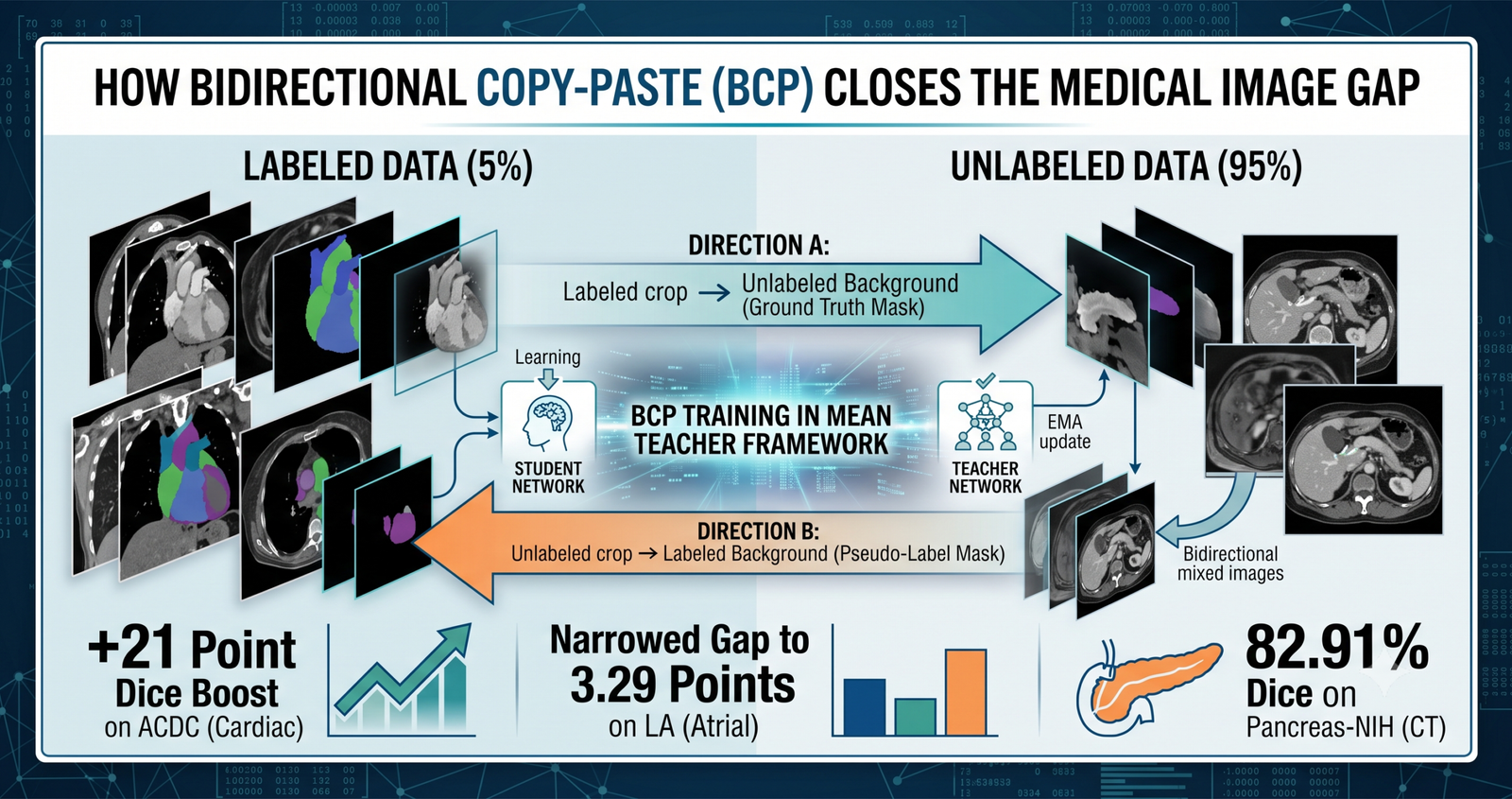
- BCP copy pastes a labeled scan crop onto an unlabeled scan and an unlabeled crop onto a labeled scan, training both directions inside a single Mean Teacher framework.
- On the ACDC cardiac dataset with only 5 percent labeled data, BCP reached 87.59 percent Dice against the next best competitor SS-Net at 65.83 percent, a gain the paper reports as over 21 percentage points.
- On the LA atrial dataset, BCP narrowed the gap between labeled and unlabeled data Dice scores to 3.29 points, compared to a gap of 7.96 points for the prior MC-Net method.
- The method adds no new trainable parameters over the underlying V-Net or U-Net backbone and keeps the same computational cost at inference time.
- These results come from three specific public research datasets under a fixed experimental protocol, not from a deployed clinical tool, and the authors themselves note the method still struggles on very low contrast structures.
The problem with treating labeled and unlabeled scans differently
Segmenting the internal structures in a CT or MRI scan, tracing the exact outline of a heart chamber, an organ, or a tumor, is essential groundwork for a long list of clinical applications, and most of the strong supervised segmentation networks that do this well need a large pool of manually labeled scans to train on. Labeling is where the real cost sits, since drawing an accurate voxel level outline on a 3D medical volume takes a trained expert real time, which is exactly why semi supervised segmentation, training on a small labeled set plus a much larger unlabeled one, has become such an active research area.
The authors frame the core difficulty as a statistics problem rather than a modeling problem. In theory, labeled and unlabeled data are drawn from the same underlying distribution. In practice, when you only have a handful of labeled scans, the empirical distribution you can actually estimate from them looks nothing like the true distribution, simply because five or ten examples cannot capture the full range of anatomical variation that a much larger unlabeled pool contains. Most existing semi supervised methods train the labeled and unlabeled branches through separate learning paths anyway, self training generates pseudo labels for the unlabeled set while the labeled set gets real ground truth, and Mean Teacher based methods apply a consistency loss to unlabeled data while treating labeled data as its own separate supervised signal. The paper’s argument is that this separation itself is the problem, because it discards a large share of what the network could have learned from labeled examples when it comes time to process unlabeled ones.
What copy paste already offered, and where it fell short
CutMix, introduced by Yun et al., established copy paste as a strong, simple augmentation technique, the idea being that pixels sitting in the same image tend to share related semantics, so blending crops from different images can teach a network more robust features than either image alone. In semi supervised learning specifically, copy paste usually gets used as a strong augmentation applied to pairs of unlabeled images, forcing a consistency loss between the weakly and strongly augmented versions.
The authors point out a narrower pattern across prior copy paste work in this space. Some methods, like the semi supervised approaches from French et al. and Kim et al., only ever copy paste between two unlabeled images. Others, echoing the instance segmentation work by Ghiasi et al., copy a crop from a labeled image as the foreground and paste it onto another image, but only ever in that one direction. Neither approach designs a genuinely consistent learning procedure that treats labeled and unlabeled data the same way, and the resulting mixed images end up supervised mostly by lower precision pseudo labels rather than the more reliable ground truth a labeled crop could provide.
How bidirectional copy paste actually works
BCP sits inside a standard Mean Teacher architecture, where a Student network is trained with gradient descent and a Teacher network is updated as an exponential moving average of the Student’s weights. Training happens in three stages. First, the authors pretrain a model using only labeled data, but with copy paste augmentation applied even at this stage, crops from one labeled image get pasted onto another labeled image. Second, this pretrained model becomes the initial Teacher network and starts generating pseudo labels for the unlabeled scans. Third, at every training iteration, the Student network is updated by stochastic gradient descent and the Teacher network is refreshed via the exponential moving average of the Student’s parameters.
The actual copy paste mechanism relies on a binary mask, sized as a fraction beta of the full volume’s height, width, and length, that marks which voxels come from a foreground image and which come from a background image. Two mixed images get generated at every step, one where a labeled crop sits inside an unlabeled background, and one where an unlabeled crop sits inside a labeled background.
Here $X_i^l$ and $X_j^l$ are two different labeled images, $X_p^u$ and $X_q^u$ are two different unlabeled images, and $M$ is the zero centered mask marking the pasted region. Using two separate labeled and two separate unlabeled images for the two mixed samples, rather than reusing the same pair twice, keeps the training signal diverse rather than repetitive.
The supervisory signal that trains the Student network follows the exact same blending logic. The Teacher network generates a probability map for each unlabeled image, which gets converted into a pseudo label through a threshold for binary tasks or an argmax operation for multi class tasks, and then cleaned up by keeping only the largest connected component to strip out stray, disconnected voxels. That cleaned pseudo label and the labeled image’s real ground truth mask get combined using the identical bidirectional blending mask used on the images themselves.
The loss function then treats the two halves of each mixed image differently, weighting the pseudo labeled portion by a factor alpha that is smaller than the weight given to the ground truth portion, since ground truth is simply more trustworthy than a pseudo label.
$L_{seg}$ here is a linear combination of Dice loss and cross entropy loss, a fairly standard choice for segmentation tasks, and $Q^{in}$ and $Q^{out}$ are simply the Student network’s predictions on the two mixed images. The total loss for a training step is just the sum of the two.
Three datasets, three different anatomical challenges
The authors tested BCP on the Left Atrium Segmentation Challenge dataset, which holds 100 3D gadolinium enhanced MRI scans of the heart’s left atrium, the Pancreas-NIH dataset, which holds 82 contrast enhanced abdominal CT volumes manually delineated for pancreas segmentation, and the ACDC dataset, a four class cardiac segmentation benchmark covering the background, right ventricle, left ventricle, and myocardium across 100 patients’ scans, split into a fixed 70, 10, and 20 patient division for training, validation, and testing. Each of these targets a genuinely different structure and imaging modality, which is a reasonable spread for testing whether a method generalizes rather than overfitting to one organ’s particular geometry.
What the numbers actually show
On the LA dataset at a 5 percent labeled ratio, four labeled scans against seventy six unlabeled ones, BCP reached 88.02 percent Dice, ahead of SS-Net at 86.33 percent, MC-Net at 83.59 percent, URPC at 82.48 percent, UA-MT at 82.26 percent, SASSNet at 81.60 percent, and DTC at 81.25 percent. At 10 percent labeled, eight scans against seventy two unlabeled, the gap narrows somewhat but BCP still leads at 89.62 percent against SS-Net’s 88.55 percent.
| Dataset | Labeled ratio | Best prior method | Prior Dice | BCP Dice |
|---|---|---|---|---|
| LA | 5 percent, 4 scans | SS-Net | 86.33 | 88.02 |
| LA | 10 percent, 8 scans | SS-Net | 88.55 | 89.62 |
| Pancreas-NIH | 20 percent, 12 scans | CoraNet | 79.67 | 82.91 |
| ACDC | 5 percent, 3 scans | SS-Net | 65.83 | 87.59 |
| ACDC | 10 percent, 7 scans | SS-Net | 86.78 | 88.84 |
The ACDC result at 5 percent labeled data is the headline number, and it deserves a closer look precisely because the jump is so large. Prior methods struggled badly at this ratio, UA-MT managed only 46.04 percent Dice, SASSNet 57.77 percent, DTC 56.90 percent, and even the strongest prior method, SS-Net, only reached 65.83 percent. BCP’s 87.59 percent represents a genuinely large jump rather than an incremental one, and the authors offer a plausible explanation, a single 3D cardiac volume can be sliced into many 2D training slices, so at very low labeled ratios there are dramatically more possible labeled and unlabeled slice combinations to draw from than there would be using full 3D volumes, letting the copy paste mechanism transfer knowledge more thoroughly exactly when labeled data is scarcest.
The overfitting signal hiding in the labeled data Dice score
One of the more interesting details in the paper is not in the main results table at all. The authors compare Dice scores separately for labeled versus unlabeled training data across several methods on the LA dataset, and the pattern is telling. MC-Net reaches 95.59 percent Dice on labeled data but only 87.63 percent on unlabeled data, a gap of 7.96 points. DTC shows a 7.13 point gap, SASSNet 7.43 points, SS-Net 6.19 points. BCP’s gap is only 3.29 points, and it gets there in an unusual way, not by pushing unlabeled performance dramatically higher than everyone else, but by having a noticeably lower labeled data Dice score of 92.88 percent compared to the 93 to 95 percent range other methods hit.
What the ablation tables reveal about which piece matters
The ablation study on copy paste direction is the clearest evidence for why bidirectional blending specifically, rather than any single direction, is doing the work. Testing inward only copy paste, unlabeled foreground onto labeled background, outward only copy paste, labeled foreground onto unlabeled background, and within set copy paste, labeled onto labeled and unlabeled onto unlabeled separately, every single variant underperforms the full bidirectional version. On ACDC at 5 percent labeled data, inward only reaches 81.68 percent Dice, outward only collapses to 72.19 percent, within set copy paste reaches 81.80 percent, and the full bidirectional method reaches 87.59 percent. That outward only result on ACDC is a particularly steep drop, with a 95 Hausdorff Distance of 39.57 voxels against BCP’s 1.90, suggesting that direction alone can produce genuinely unstable boundary predictions.
The masking shape ablation is similarly informative. A random mask made of many small scattered zero value cubes performed worst, since scattered small crops only capture incoherent local fragments of the foreground rather than a complete representation of it. A contact mask, shaped as a full slab through part of the volume, did better by preserving more foreground integrity, reaching 86.64 percent Dice at the 5 percent labeled ratio on LA. The zero centered cube mask BCP actually uses reached 88.02 percent, which the authors attribute to giving the foreground more surface area to interact with the surrounding background compared to a mask sitting flush against one edge.
The stepwise breakdown on ACDC at 5 percent labeled data is the most granular accounting in the paper. A baseline pseudo label self training approach with none of BCP’s components reaches only 47.62 percent Dice. Adding the bidirectional copy paste mechanism alone jumps that to 83.26 percent, the single largest jump in the whole ablation chain. Adding non maximum suppression style post processing on the pseudo labels actually produces a small Dice dip, to 82.33 percent, though it substantially improves the 95 Hausdorff Distance from 23.90 down to 9.78, suggesting it trades a small amount of overlap accuracy for much better boundary stability. Finally, initializing the Teacher network from a model pretrained with copy paste, rather than a randomly initialized one or one pretrained without copy paste, pushes the final result to 87.59 percent Dice and a much tighter 1.90 Hausdorff Distance.
| Configuration on ACDC, 5 percent labeled | Dice | 95HD |
|---|---|---|
| No BCP components, plain pseudo label self training | 47.62 | 29.02 |
| Add bidirectional copy paste | 83.26 | 23.90 |
| Add pseudo label post processing | 82.33 | 9.78 |
| Add copy paste based pretraining, the full method | 87.59 | 1.90 |
That table is a genuinely useful piece of transparency. The bidirectional copy paste mechanism itself accounts for the overwhelming majority of the improvement, roughly 36 percentage points of Dice out of the total 40 point jump from baseline to final, while post processing and better pretraining refine boundary quality more than raw overlap accuracy. Anyone trying to reproduce a slice of this result rather than the whole pipeline should know that the copy paste mechanism, not the auxiliary tricks around it, is where the real gain lives.
Two more ablations round out the picture. Comparing BCP against Mixup, which superimposes whole images rather than pasting crops, and against a fine grained CutMix variant that chops images into a four by four grid of patches, both alternatives perform substantially worse, Mixup collapsing to 41.71 percent Dice at 5 percent labeled data on LA and fine grained CutMix reaching 67.05 percent, against BCP’s 88.02 percent. The authors attribute Mixup’s weak showing to the fact that superimposing two full medical images introduces more structural noise than blending across whole images tends to introduce in natural photographs, where the technique originated. The loss weighting parameter alpha, which controls how much a pseudo labeled region contributes to the loss relative to a ground truth region, turned out to be fairly forgiving between 0.5 and 1.5 but showed a clear performance drop at 2.5, and the mask size ratio beta performed best at two thirds of the volume dimension, with performance falling off at both smaller and, to a lesser extent, larger ratios.
Clinical translation gap
It is worth being precise about what these numbers do and do not demonstrate. LA, Pancreas-NIH, and ACDC are all established, curated research benchmarks built specifically to let different semi supervised methods be compared under an identical protocol. That is genuinely valuable for methodological research, since it lets a result like BCP’s ACDC jump be attributed to the method rather than to differences in preprocessing or evaluation across papers. But a benchmark built for fair comparison is a different thing from a tool validated for use in an actual radiology or cardiology workflow.
None of the three datasets in this paper represent a prospective clinical deployment. They are retrospective collections of scans, gathered under a specific research protocol with specific scanners and specific patient populations, and the paper reports results on a single fixed train, validation, and test split per dataset rather than across multiple independent institutions or scanner types. The ACDC experiments in particular train on 2D slices extracted from 3D volumes, which is a reasonable and common way to increase the number of possible training combinations at very low labeled ratios, but it also means the model never directly reasons about full 3D spatial continuity during that particular set of experiments, only about individual 2D cross sections, which is a real architectural choice with real tradeoffs for a genuinely 3D anatomical structure like a beating heart.
The authors are also candid, in their own limitations paragraph, that BCP was not specifically designed with a module for learning local, fine grained attributes, and that even their best configuration still struggles to segment low contrast target regions well, pointing to a specific visible gap in one of their own result figures. That kind of self reported failure case is exactly the sort of detail worth taking seriously rather than treating the headline Dice numbers as the whole story.
Clinical and technical limitations worth sitting with
A few specific points deserve to be named directly rather than folded into a general caveat. The reported gains, while large and consistent across three datasets, come from fixed random seeds on single train and test splits, so the exact percentage improvements over competitors, some as narrow as roughly one Dice point at the 10 percent labeled ratios, should be read with some caution about how much they would vary under repeated runs or cross validation. The Pancreas-NIH result at 20 percent labeled data represents a considerably higher labeled ratio than the ACDC experiments at 5 percent, so the two headline numbers, an over 21 point Dice improvement on ACDC and a roughly 3 point improvement on Pancreas-NIH, are not directly comparable achievements, they reflect very different starting points for how much labeled data was already available.
The method’s own authors flag that low contrast structures remain a specific weak point, visible in their own qualitative figure where a portion of a target organ is missed entirely under their best configuration. And while the paper reports strong Hausdorff Distance and Average Surface Distance numbers, meaning the boundaries BCP produces tend to be spatially closer to the ground truth than competing methods, none of these geometric accuracy metrics say anything about how a clinician would actually use this output, whether as a fully automated segmentation, a starting point for manual correction, or a second opinion alongside their own reading of the scan. That downstream question is simply outside the scope of what this paper tested.
Why this still matters despite the caveats
Strip away the clinical translation question and look at this as a training methodology contribution, and the case for BCP is genuinely strong. It adds zero new trainable parameters over a standard V-Net or U-Net backbone, meaning any team already running one of those architectures could adopt bidirectional copy paste as a training procedure change rather than an architecture change, without paying any additional inference cost. That is a meaningfully lower barrier to adoption than most competing methods in this space, several of which add dedicated uncertainty estimation modules, auxiliary tasks, or additional network branches that increase both training complexity and inference cost.
Full conclusion
The core achievement here is showing that a genuinely simple mechanism, blending labeled and unlabeled scans onto each other in both directions and carrying that same blending logic through to the supervisory signal, closes a documented empirical distribution gap that more architecturally elaborate prior methods left largely unaddressed. The ablation tables back this up with real granularity rather than a single aggregate number, showing that the bidirectional mechanism itself, not auxiliary tricks layered on top of it, accounts for the overwhelming share of the improvement on the hardest tested setting.
The conceptual shift worth remembering is narrower than the eye catching 21 point Dice jump on ACDC. This is not a claim that copy paste augmentation solves semi supervised segmentation broadly. It is a demonstration that the direction and symmetry of how you blend labeled and unlabeled data matters more than previously appreciated, and that treating both directions consistently, rather than picking one, is what actually narrows the distribution gap the paper opens with.
Whether this transfers cleanly to other domains is a reasonable question given how the method was tested. The three datasets used here, cardiac MRI, atrial MRI, and pancreatic CT, all share fairly compact, well defined anatomical targets against a comparatively homogeneous background. Structures with more diffuse boundaries, more variable background context, or more subtle intensity differences from surrounding tissue, exactly the low contrast case the authors themselves flag as a remaining weakness, may not benefit as cleanly, and that is a real open question the paper leaves for future work rather than one it answers.
The honest remaining limitations are the ones already laid out above and should not be softened. Results rest on single splits with fixed seeds rather than repeated cross validation. The labeled ratios tested differ meaningfully across datasets, so headline improvement percentages should not be compared directly across them. And the authors’ own stated weakness, difficulty with low contrast targets, is a real, acknowledged gap rather than a hypothetical one.
Put simply, BCP is a well ablated, parameter free training procedure that measurably narrows a real and previously underaddressed distribution gap in semi supervised medical image segmentation, tested carefully across three separate anatomical targets. It is not, and does not claim to be, a validated clinical segmentation tool, and reading it as the former rather than the latter is the accurate way to take both its real contribution and its real limits seriously at the same time.
Reference implementation in PyTorch
The code below is an independent, simplified implementation of the bidirectional copy paste mechanism and the Mean Teacher training loop described in Section 3 of the paper, wired onto a small 3D convolutional segmentation network so the whole pipeline can run end to end as a smoke test on dummy data. It is not the authors’ original code, which the authors have published separately, and it uses a lightweight backbone rather than the paper’s full V-Net or U-Net to keep the example runnable and focused on the copy paste and loss mechanism that is the actual contribution of this paper.
# bcp_reference.py
# Independent reference implementation of Bidirectional Copy Paste
# for semi supervised segmentation, following Equations 1 through 9
# in the source paper. Uses a compact 3D CNN backbone rather than the
# paper's full V-Net or U-Net to keep the smoke test lightweight.

import torch
import torch.nn as nn
import torch.nn.functional as F
import copy


class SmallSegNet(nn.Module):
    """A compact 3D encoder decoder segmentation network, standing in
    for the paper's V-Net or U-Net backbone."""

    def __init__(self, in_channels=1, num_classes=2, base=8):
        super().__init__()
        self.enc1 = nn.Sequential(
            nn.Conv3d(in_channels, base, 3, padding=1), nn.ReLU(inplace=True)
        )
        self.enc2 = nn.Sequential(
            nn.Conv3d(base, base * 2, 3, stride=2, padding=1), nn.ReLU(inplace=True)
        )
        self.dec1 = nn.Sequential(
            nn.ConvTranspose3d(base * 2, base, 2, stride=2), nn.ReLU(inplace=True)
        )
        self.out_conv = nn.Conv3d(base, num_classes, 1)

    def forward(self, x):
        f1 = self.enc1(x)
        f2 = self.enc2(f1)
        d1 = self.dec1(f2)
        return self.out_conv(d1 + f1)


def make_zero_centered_mask(shape, beta=2 / 3, device="cpu"):
    """Builds the zero centered mask M from Section 3.1.3. Ones
    everywhere except a centered cube sized beta times each dimension,
    which is zero, marking where the background image shows through."""
    _, _, d, h, w = shape
    mask = torch.ones(shape, device=device)
    zd, zh, zw = int(d * beta), int(h * beta), int(w * beta)
    d0, h0, w0 = (d - zd) // 2, (h - zh) // 2, (w - zw) // 2
    mask[:, :, d0:d0 + zd, h0:h0 + zh, w0:w0 + zw] = 0
    return mask


def bidirectional_copy_paste(labeled_i, labeled_j, unlabeled_p, unlabeled_q, mask):
    """Equations 1 and 2. Builds the inward and outward mixed images."""
    x_in = labeled_j * mask + unlabeled_p * (1 - mask)
    x_out = unlabeled_q * mask + labeled_i * (1 - mask)
    return x_in, x_out


def bidirectional_copy_paste_labels(label_j, pseudo_p, pseudo_q, label_i, mask):
    """Equations 4 and 5. Blends ground truth and pseudo labels using
    the exact same mask used for the images themselves."""
    y_in = label_j * mask + pseudo_p * (1 - mask)
    y_out = pseudo_q * mask + label_i * (1 - mask)
    return y_in, y_out


def dice_loss(logits, targets, num_classes, eps=1e-6):
    """Soft Dice loss across all classes, one half of the Lseg
    combination described in Section 3.2."""
    probs = F.softmax(logits, dim=1)
    targets_onehot = F.one_hot(targets, num_classes=num_classes)
    targets_onehot = targets_onehot.permute(0, 4, 1, 2, 3).float()

    dims = (0, 2, 3, 4)
    intersection = (probs * targets_onehot).sum(dims)
    union = probs.sum(dims) + targets_onehot.sum(dims)
    dice_per_class = (2 * intersection + eps) / (union + eps)
    return 1 - dice_per_class.mean()


def seg_loss(logits, targets, num_classes):
    """Lseg, the linear combination of Dice loss and cross entropy
    loss used throughout the paper's loss function."""
    ce = F.cross_entropy(logits, targets)
    dsc = dice_loss(logits, targets, num_classes)
    return 0.5 * ce + 0.5 * dsc


def masked_bcp_loss(logits, targets, mask, alpha=0.5, num_classes=2, invert=False):
    """Equations 6 and 7. Weights the ground truth region at full
    strength and the pseudo labeled region by alpha. Set invert True
    for the outward mixed image, where the mask meaning flips."""
    mask_1ch = mask[:, 0:1].expand_as(targets.unsqueeze(1)).squeeze(1)
    strong_region = mask_1ch if not invert else (1 - mask_1ch)
    weak_region = 1 - strong_region

    per_voxel_ce = F.cross_entropy(logits, targets, reduction="none")
    weighted = per_voxel_ce * strong_region + alpha * per_voxel_ce * weak_region
    ce_term = weighted.mean()

    dsc_term = dice_loss(logits, targets, num_classes)
    return 0.5 * ce_term + 0.5 * dsc_term


def update_teacher(teacher, student, ema_decay=0.99):
    """Equation 10. Exponential moving average update of the Teacher
    network's parameters from the Student network's parameters."""
    with torch.no_grad():
        for t_param, s_param in zip(teacher.parameters(), student.parameters()):
            t_param.data.mul_(ema_decay).add_(s_param.data, alpha=1 - ema_decay)


def run_smoke_test():
    """Runs a short training loop on random dummy 3D volumes, shaped
    like a small cardiac MRI patch, to confirm the copy paste
    mechanism, loss function, and Teacher update all run end to end."""
    torch.manual_seed(0)
    num_classes = 4  # matches the four ACDC classes
    shape = (1, 1, 16, 32, 32)  # batch, channel, depth, height, width

    student = SmallSegNet(in_channels=1, num_classes=num_classes)
    teacher = copy.deepcopy(student)
    for p in teacher.parameters():
        p.requires_grad_(False)

    optimizer = torch.optim.SGD(student.parameters(), lr=0.01)

    for step in range(3):
        labeled_i = torch.randn(shape)
        labeled_j = torch.randn(shape)
        unlabeled_p = torch.randn(shape)
        unlabeled_q = torch.randn(shape)
        label_i = torch.randint(0, num_classes, shape[0:1] + shape[2:])
        label_j = torch.randint(0, num_classes, shape[0:1] + shape[2:])

        # Teacher generates pseudo labels for the two unlabeled volumes
        with torch.no_grad():
            pseudo_p = torch.argmax(teacher(unlabeled_p), dim=1)
            pseudo_q = torch.argmax(teacher(unlabeled_q), dim=1)

        mask = make_zero_centered_mask(shape, beta=2 / 3)

        x_in, x_out = bidirectional_copy_paste(labeled_i, labeled_j, unlabeled_p, unlabeled_q, mask)
        y_in, y_out = bidirectional_copy_paste_labels(label_j, pseudo_p, pseudo_q, label_i, mask)

        q_in = student(x_in)
        q_out = student(x_out)

        loss_in = masked_bcp_loss(q_in, y_in, mask, alpha=0.5, num_classes=num_classes, invert=False)
        loss_out = masked_bcp_loss(q_out, y_out, mask, alpha=0.5, num_classes=num_classes, invert=True)
        loss = loss_in + loss_out

        optimizer.zero_grad()
        loss.backward()
        optimizer.step()
        update_teacher(teacher, student, ema_decay=0.99)

        print(f"step {step} loss {loss.item():.4f}")

    assert q_in.shape == (1, num_classes, 16, 32, 32), "unexpected output shape"
    print("smoke test passed")


if __name__ == "__main__":
    run_smoke_test()
Read the full paper for the complete tables, figures, and supplementary ablation study
Read the paper on arXiv Official BCP code repositoryFrequently asked questions
What is Bidirectional Copy Paste
BCP is a training method for semi supervised medical image segmentation that copy pastes a crop from a labeled scan onto an unlabeled scan and a crop from an unlabeled scan onto a labeled scan, training both directions together inside a Mean Teacher architecture to close the gap between how the model handles labeled versus unlabeled data.
How much better is BCP than prior methods
On the ACDC cardiac dataset with only 5 percent labeled data, BCP reached 87.59 percent Dice against the next best competitor at 65.83 percent, an improvement the paper reports as over 21 percentage points. Gains on the LA atrial and Pancreas-NIH pancreatic datasets were smaller but still consistently ahead of prior state of the art methods.
Does BCP require a bigger or more complex network
No. The paper reports that BCP adds no new trainable parameters over the underlying V-Net or U-Net backbone and keeps the same computational cost, since it changes how training data is constructed and supervised rather than changing the network architecture itself.
What datasets was BCP tested on
Three public research datasets, the Left Atrium Segmentation Challenge dataset with 100 cardiac MRI scans, the Pancreas-NIH dataset with 82 abdominal CT volumes, and the ACDC dataset with 100 patients’ cardiac MRI scans across four segmentation classes.
Is BCP a clinical diagnostic tool
No. This is a research method evaluated on curated benchmark datasets under a fixed research protocol. It has not been validated in a prospective clinical setting, has not gone through regulatory review, and the authors themselves note it still struggles with low contrast target regions.
What are the main limitations of this study
Results come from single train and test splits with fixed random seeds rather than repeated cross validation, the labeled data ratios tested differ across datasets so headline improvement percentages are not directly comparable, and the authors report that very low contrast structures remain difficult to segment even with the full method.
Related reading in this pillar
Bai, Y., Chen, D., Li, Q., Shen, W., and Wang, Y. (2023). Bidirectional copy paste for semi supervised medical image segmentation. arXiv:2305.00673. Code available at https://github.com/DeepMed-Lab-ECNU/BCP
This analysis is based on the published paper and an independent evaluation of its claims.