
Key points
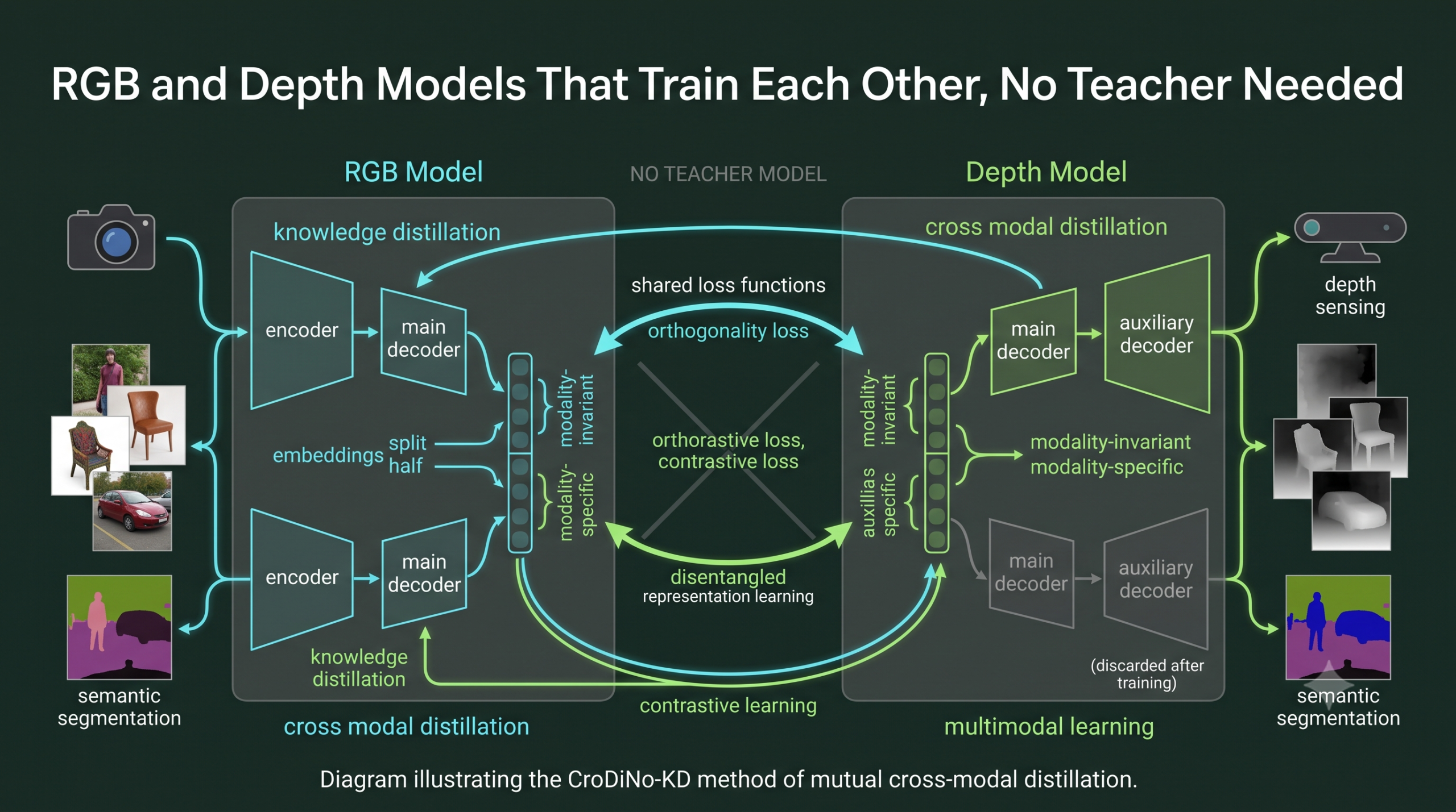
- CroDiNo-KD drops the multimodal teacher entirely and instead trains an RGB model and a Depth model together, letting them shape each other through shared loss functions during training.
- Each model’s internal representation is deliberately split into a modality invariant half and a modality specific half, using disentanglement learning, contrastive learning, and an auxiliary decoder that gets thrown away after training.
- Because there is no teacher demanding matched inputs, RGB and Depth images can be augmented independently rather than in lockstep, a flexibility the paper calls decoupled augmentation.
- Across three RGBD segmentation benchmarks spanning indoor scenes, aerial imagery, and drone footage, CroDiNo-KD is the only method tested that improves over a plain single modality baseline in every single one of six test scenarios.
- On the Potsdam remote sensing benchmark, several well established distillation baselines actually score worse than training no distillation at all, while CroDiNo-KD’s RGB model, remarkably, outperforms the full multimodal teacher it never even had.
- Because it skips teacher pretraining, CroDiNo-KD trains in roughly half the total time and less than half the parameter count of the cheapest teacher based competitor tested.
The core problem, the teacher itself is part of the overhead
Cross modal knowledge distillation for RGBD data almost always follows the same recipe. Train a multimodal teacher that consumes both RGB and Depth, then train one or more single modality student models to mimic what that teacher learned, so the student can operate later using only the modality it will actually have access to at inference time. It is a sensible idea, and it works, but the paper’s authors point out two costs that come bundled with it. First, the approach is sensitive to a whole set of design choices that have nothing to do with the actual segmentation task, which teacher architecture to use, how to fuse the two modalities inside that teacher, and which specific distillation technique to apply, each of which can swing results in ways that are hard to predict ahead of time. Second, and more concretely, the standard recipe requires training and storing an entire extra model, the multimodal teacher, on top of every single modality student needed for deployment, which adds real computational cost that scales with however many target modalities a project needs to support.
CroDiNo-KD, short for Cross-Modal Disentanglement, a New Outlook on Knowledge Distillation, questions whether the teacher is even necessary. Instead of training a multimodal model first and distilling from it afterward, the framework trains the RGB and Depth models side by side, from the start, letting them influence each other through carefully designed loss functions rather than through an explicit teaching relationship. No architecture has to be chosen for a teacher that will not exist. No fusion mechanism needs designing. And only two models get trained instead of three.
Where this idea comes from
Knowledge distillation itself traces back to work by Hinton and colleagues, who formalized transferring a large teacher model’s soft predictions into a smaller student via a Kullback-Leibler divergence term, typically combined with the student’s own task loss. Extending this across modalities, rather than just across model sizes, has become its own active line of research, and for semantic segmentation specifically, several recent approaches have layered increasingly elaborate machinery onto the basic teacher and student relationship, generative reconstruction tasks, prototype based similarity transfer, and angular constraints on features, among others, all still built around a multimodal teacher handing information down.
The specific idea CroDiNo-KD builds on, disentanglement representation learning, comes from a different tradition. Rather than compressing a representation down to whatever a task needs, disentanglement deliberately splits a representation into separate, semantically meaningful pieces, in this case a piece that should look the same regardless of which modality produced it, and a piece that should capture whatever is unique to that specific modality. The paper credits a prior work by two of its own authors, applying disentanglement together with adversarial learning to cross modal distillation for scene classification, as the direct inspiration, and frames the current paper as extending that idea from a single image label per photo to the much denser, pixel by pixel demands of semantic segmentation.
How CroDiNo-KD actually works
The architecture consists of two complete encoder-decoder models, one for RGB and one for Depth, plus a third auxiliary decoder that only exists during training and gets discarded afterward. Each modality’s encoder produces an embedding that is split down the middle into two equally sized halves.
Encoding each modality, then splitting the representation in half
$$Z_m = \mathrm{Enc}_m(X_m), \quad m \in \{RGB, D\}, \qquad Z_m \rightarrow \big(Z_m^{inv},\ Z_m^{spc}\big)$$The invariant half, $Z_m^{inv}$, is pushed during training to encode information that should look similar no matter which modality produced it. The specific half, $Z_m^{spc}$, is left to capture whatever is unique to that particular sensor. The main decoder for each modality always receives both halves concatenated together, matching how the model will actually run at inference time.
Feature mixup, borrowing a bit of the other modality
To actively encourage the invariant halves to behave consistently across modalities, CroDiNo-KD blends them together before decoding, controlled by a mixing strength $\lambda$.
Blending the invariant embeddings across modalities
$$\tilde{Z}_{RGB}^{inv} = \lambda Z_D^{inv} + (1-\lambda) Z_{RGB}^{inv}, \qquad \tilde{Z}_D^{inv} = \lambda Z_{RGB}^{inv} + (1-\lambda) Z_D^{inv}$$Both the original and the blended embeddings get decoded and both contribute to the segmentation loss, which means each model has to remain accurate even when part of its invariant signal has effectively been swapped in from the other sensor.
Four loss terms doing four different jobs
The segmentation loss is standard, pixel wise cross entropy comparing each modality’s prediction against the ground truth labels.
The main segmentation loss for modality m
$$\mathcal{L}_{seg}^{m} = CE\big(\mathrm{Dec}_m([Z_m^{inv} : Z_m^{spc}]),\ Y\big)$$An orthogonality loss then pushes each modality’s own invariant and specific halves apart, using cosine similarity as the penalty, so the two halves are discouraged from encoding redundant information.
Orthogonality between a modality’s own invariant and specific embeddings
$$\mathcal{L}_{\perp}^{m} = \frac{1}{B}\sum_{b=1}^{B}\sum_{i=1}^{h}\sum_{j=1}^{w} \mathrm{sim}\big(Z_m^{inv}[b,i,j,:],\ Z_m^{spc}[b,i,j,:]\big)$$A contrastive loss, built on InfoNCE with a negative Euclidean distance in place of the more common dot product, pulls the pooled, normalized invariant embeddings of the same instance across both modalities toward each other while pushing every other embedding in the batch away.
The contrastive loss anchored on the RGB modality, with an analogous term anchored on Depth
$$\mathcal{L}_{con}^{RGB} = -\frac{1}{B}\sum_{i=1}^{B} \log \frac{\exp(-\lVert p_{RGB}^{(i)} – p_D^{(i)} \rVert_2 / \tau)}{\sum_{m \in \{RGB,D\}} \sum_{j \neq i} \exp(-\lVert p_{RGB}^{(i)} – p_m^{(j)} \rVert_2 / \tau)}$$Finally, the auxiliary decoder, the piece of the architecture that gets thrown away once training finishes, is fed the invariant and specific halves one at a time, never together, forcing each half on its own to carry enough information to be useful for segmentation.
The auxiliary loss, applied to each half of the embedding separately
$$\mathcal{L}_{aux}^{m} = CE\big(\mathrm{Dec}_{Aux}(Z_m^{inv}),\ Y\big) + CE\big(\mathrm{Dec}_{Aux}(Z_m^{spc}),\ Y\big)$$All four terms, across both modalities, are simply added together with no weighting coefficients at all.
The total training objective, an unweighted sum of everything above
$$\mathcal{L}_{tot} = \sum_{m \in \{RGB, D\}} \Big(\mathcal{L}_{con}^{m} + \mathcal{L}_{seg}^{m} + \mathcal{L}_{\perp}^{m} + \mathcal{L}_{aux}^{m}\Big)$$That absence of tunable loss weights is a small detail with a real practical upside. Most multi loss training setups need at least some hyperparameter search just to find weights that keep every term contributing rather than one term drowning out the others, and CroDiNo-KD sidesteps that search entirely.
Decoupled augmentation, a freedom the teacher never allowed
Conventional teacher and student pipelines typically need the RGB and Depth inputs to go through matched, paired augmentations, since the teacher processes both together and any mismatch between them would corrupt what it learns. Because CroDiNo-KD computes RGB and Depth losses separately rather than fusing the two modalities anywhere in the training loop, it can augment each modality independently, flipping, scaling, or cropping RGB and Depth images on their own schedules rather than in lockstep, and adding color jitter to RGB only, since that transformation has no sensible analogue for a depth map.
What the experiments actually show
The authors test CroDiNo-KD on three RGBD segmentation benchmarks chosen specifically to span different domains, NYU Depth v2 for indoor scenes captured with a Kinect sensor, Potsdam for aerial remote sensing imagery paired with elevation data, and Mid-Air, a synthetic dataset of low altitude drone flight footage with stereo depth. Competing methods include a plain single modality baseline with no distillation at all, the full multimodal teacher itself, two standard knowledge distillation baselines, and four more recent, purpose built cross modal distillation frameworks, KD-Net, Masked Generative Distillation, ProtoKD, and two angular distillation variants called LAD and CAD.
| Model | NYUDepth RGB | NYUDepth Depth | Potsdam RGB | Potsdam Depth | Mid-Air RGB | Mid-Air Depth |
|---|---|---|---|---|---|---|
| single modality | 42.64 | 36.01 | 75.73 | 42.47 | 47.84 | 47.07 |
| KDv1 | 43.43 up | 36.44 up | 66.32 down | 39.20 down | 47.36 down | 45.80 down |
| KD-Net | 42.78 up | 36.36 up | 73.82 down | 41.85 down | 48.32 up | 46.22 down |
| Masked Dist. | 40.97 down | 34.93 down | 76.09 up | 42.43 down | 47.60 down | 47.40 up |
| CroDiNo-KD | 44.85 up | 37.60 up | 76.13 up | 42.78 up | 48.37 up | 47.91 up |
Two results here deserve more attention than the paper gives them in passing. The first is what happens to the established baselines on Potsdam. KDv1 scores 66.32 there against a single modality baseline of 75.73, a drop of more than nine points, and the pattern repeats for KD-Net, ProtoKD, LAD, and CAD, every one of which underperforms a model trained with no distillation supervision whatsoever on that specific dataset. These are not weak or unusual methods, they are established techniques that work reasonably well on the other two benchmarks, which suggests something about the Potsdam domain, likely its unusual four channel remote sensing imagery and elevation based depth signal, breaks assumptions that these methods were built around. That is a genuinely useful, somewhat uncomfortable finding for anyone assuming a published distillation method will transfer safely to a new domain without checking first.
The second result is stranger still. On Potsdam, CroDiNo-KD’s RGB model reaches 76.13 mIoU, and Masked Dist.’s RGB model reaches 76.09, both of which exceed the full multimodal teacher’s own score of 74.98. A single modality student beating the multimodal teacher it was supposed to be learning from is not something the standard teacher and student framing has an easy explanation for, and it is a useful reminder that a fused multimodal model is not automatically the ceiling on what a well trained single modality model can achieve, especially when the fusion mechanism itself may not be well suited to the specific domain in question.
Across all six RGB and Depth combinations tested, CroDiNo-KD is the only method that improves over the single modality baseline in every single case. Every other method tested, including both standard KD baselines and every purpose built CMKD competitor, underperforms the baseline in at least one of the six scenarios.
Key takeaway
Several well regarded cross modal distillation methods actively hurt performance relative to training no distillation at all on at least one of the three benchmarks tested here. Consistency across domains, not just peak performance on a familiar benchmark, is the harder and more relevant bar to clear.What the ablation and sensitivity results add
Removing each of CroDiNo-KD’s four loss terms one at a time confirms that every component earns its place, with the auxiliary loss and the contrastive loss causing the largest drops in average mIoU when removed, 49.09 and 49.11 respectively against the full model’s 49.61. Removing the feature mixup step causes the smallest drop of the five ablations tested, 49.31, suggesting it is a genuine but comparatively minor contributor next to the disentanglement and contrastive machinery doing most of the heavy lifting.
A separate sweep of the mixup strength $\lambda$ from 0.05 to 0.5 finds broadly stable performance across that range, with one exception worth flagging. The standard deviation on Mid-Air’s Depth column is 0.44, three to four times larger than the standard deviation reported for any other column in that sweep. The paper’s overall claim of stability across the tested range holds up reasonably well for five of the six reported columns, but that one column is meaningfully noisier than the rest, and is worth keeping in mind before assuming the mixup hyperparameter is equally forgiving in every setting.
Where the real advantage shows up, training cost
The efficiency numbers are where CroDiNo-KD’s design choice to skip the teacher pays off most clearly and most concretely. On the Mid-Air dataset, training both the RGB and Depth single modality models with CroDiNo-KD takes 20 hours and 30 minutes total, with zero teacher pretraining overhead since no teacher exists. Every teacher based competitor tested carries an identical extra 14 hours of teacher pretraining on top of its own distillation time, pushing the cheapest of them, KDv1 and KDv2, to 36 hours total, and the most expensive, Masked Generative Distillation, all the way to 61 hours and 22 minutes, roughly three times CroDiNo-KD’s total.
Parameter counts tell a similar story. CroDiNo-KD’s main architecture uses 68 million parameters, smaller than every competitor’s 80 million, since the framework deliberately narrows the encoder’s output to accommodate the disentanglement split. Its lightweight auxiliary decoder adds only 5 million more, for a training time total of 73 million parameters. Every teacher based competitor, by contrast, needs to also store a 98 million parameter teacher during training, and the worst case, Masked Dist., needs a further 150 million parameters for its generative auxiliary decoder, bringing its training time total to 328 million parameters, well over four times CroDiNo-KD’s footprint.
Honest limitations of this study
The paper is a solid empirical contribution, and a close read still turns up some real caveats worth keeping in mind.
- All three benchmarks use only two modalities, RGB and Depth. Whether the same disentanglement and contrastive machinery scales cleanly to three or more modalities, where the notion of a single shared invariant space becomes considerably harder to define, is not tested here.
- The framework’s headline claim of stability across the mixup hyperparameter range is largely well supported, but the Mid-Air Depth column shows meaningfully higher variance than every other column in that sweep, a detail easy to miss if a reader only skims the paper’s summary sentence rather than the actual standard deviation row in the table.
- The paper reports a single run’s mIoU per method per benchmark in the main results table, without confidence intervals or repeated runs, which makes it hard to know how much of the sometimes narrow gap over the strongest competitor, such as the 0.04 point margin over Masked Dist. on Potsdam RGB, reflects a genuine, reproducible advantage versus run to run noise.
- Every comparison uses the same ResNet-50 and DeepLabV3+ backbone architecture across all methods, which is a fair way to isolate the effect of the distillation strategy itself, but it also means the results say nothing about how CroDiNo-KD’s relative advantage might change with a different or larger backbone.
- The striking result of several baselines underperforming the no distillation baseline on Potsdam is reported but not deeply investigated. The paper does not dig into why that specific domain breaks those specific methods, leaving a genuinely interesting open question for follow up work.
Reference implementation, CroDiNo-KD’s core losses in PyTorch
The snippet below is a compact, runnable stand in for CroDiNo-KD’s encoder and decoder structure, the four loss terms, and one full training step matching Algorithm 1 in the paper. It uses tiny random image tensors and a small number of segmentation classes so it runs anywhere without a real dataset or checkpoint, and it has been executed end to end across several optimizer steps to confirm the loss decreases and produces no errors.
# -----------------------------------------------------------------------
# Educational reference implementation inspired by CroDiNo-KD, described
# in Ferrod et al., "Revisiting Cross-Modal Knowledge Distillation, A
# Disentanglement Approach for RGBD Semantic Segmentation" (arXiv
# 2505.24361). It illustrates, on tiny dummy tensors, the four loss
# terms and the joint training loop that let two single-modality models
# teach each other without any multi-modal teacher.
#
# Note on tensor layout: the paper writes tensors channels-last
# (B x H x W x C). This implementation uses PyTorch's standard
# channels-first (B x C x H x W) layout instead, which is
# mathematically equivalent.
# -----------------------------------------------------------------------

import torch
import torch.nn as nn
import torch.nn.functional as F


# -------------------------------------------------------------------
# 1. A small per-modality encoder, Equation 2. Maps an RGB or Depth
#    image to an embedding with F channels, later split in half into
#    modality-invariant and modality-specific halves.
# -------------------------------------------------------------------
class SimpleEncoder(nn.Module):
    def __init__(self, in_channels, embed_channels):
        super().__init__()
        self.net = nn.Sequential(
            nn.Conv2d(in_channels, 32, kernel_size=3, padding=1),
            nn.ReLU(),
            nn.Conv2d(32, embed_channels, kernel_size=3, padding=1),
        )

    def forward(self, x):
        z = self.net(x)
        half = z.size(1) // 2
        z_inv, z_spc = z[:, :half], z[:, half:]
        return z_inv, z_spc


# -------------------------------------------------------------------
# 2. The main decoder, used at inference time. Takes the concatenated
#    invariant and specific embeddings and produces per pixel class
#    logits, matching the [Z_inv : Z_spc] input in Equation 4.
# -------------------------------------------------------------------
class SimpleDecoder(nn.Module):
    def __init__(self, embed_channels, num_classes):
        super().__init__()
        self.net = nn.Sequential(
            nn.Conv2d(embed_channels, 32, kernel_size=3, padding=1),
            nn.ReLU(),
            nn.Conv2d(32, num_classes, kernel_size=1),
        )

    def forward(self, z_inv, z_spc):
        z = torch.cat([z_inv, z_spc], dim=1)
        return self.net(z)


# -------------------------------------------------------------------
# 3. The auxiliary decoder, discarded after training. It only ever sees
#    one half of an embedding at a time, forcing that half alone to
#    carry enough information for segmentation, matching Equation 8.
# -------------------------------------------------------------------
class AuxDecoder(nn.Module):
    def __init__(self, half_channels, num_classes):
        super().__init__()
        self.net = nn.Sequential(
            nn.Conv2d(half_channels, 16, kernel_size=3, padding=1),
            nn.ReLU(),
            nn.Conv2d(16, num_classes, kernel_size=1),
        )

    def forward(self, z_half):
        return self.net(z_half)


# -------------------------------------------------------------------
# 4. Feature mixup, Equation 3. Blends the invariant embeddings of the
#    two modalities so each model also learns to decode a partially
#    "borrowed" invariant representation.
# -------------------------------------------------------------------
def feature_mixup(z_inv_self, z_inv_other, lam):
    return lam * z_inv_other + (1 - lam) * z_inv_self


# -------------------------------------------------------------------
# 5. The orthogonality loss, Equation 5. Pushes each modality's
#    invariant and specific embeddings toward low cosine similarity, so
#    the two halves are encouraged to encode complementary information.
# -------------------------------------------------------------------
def orthogonality_loss(z_inv, z_spc):
    z_inv_flat = z_inv.permute(0, 2, 3, 1).reshape(-1, z_inv.size(1))
    z_spc_flat = z_spc.permute(0, 2, 3, 1).reshape(-1, z_spc.size(1))
    cos_sim = F.cosine_similarity(z_inv_flat, z_spc_flat, dim=-1, eps=1e-8)
    return cos_sim.mean()


# -------------------------------------------------------------------
# 6. The contrastive loss, Equations 6 and 7. Spatially pools and L2
#    normalizes each modality's invariant embedding into one vector per
#    instance, then pulls RGB and Depth vectors of the same instance
#    together with an InfoNCE style loss based on negative distance.
# -------------------------------------------------------------------
def pooled_and_normalized(z_inv):
    pooled = z_inv.mean(dim=(2, 3))
    return F.normalize(pooled, dim=-1, eps=1e-8)


def contrastive_loss(p_rgb, p_depth, temperature=0.07):
    batch_size = p_rgb.size(0)
    all_p = torch.cat([p_rgb, p_depth], dim=0)
    distances = torch.cdist(all_p, all_p, p=2)
    logits = -distances / temperature

    mask = torch.eye(2 * batch_size, dtype=torch.bool, device=p_rgb.device)
    logits = logits.masked_fill(mask, float("-inf"))

    total_loss = 0.0
    for anchor_idx in range(batch_size):
        positive_idx = anchor_idx + batch_size
        total_loss += F.cross_entropy(
            logits[anchor_idx].unsqueeze(0), torch.tensor([positive_idx], device=p_rgb.device)
        )
        total_loss += F.cross_entropy(
            logits[positive_idx].unsqueeze(0), torch.tensor([anchor_idx], device=p_rgb.device)
        )
    return total_loss / (2 * batch_size)


# -------------------------------------------------------------------
# 7. One full training step, matching Algorithm 1. Both modalities are
#    encoded, mixed up, decoded through the main and auxiliary
#    decoders, and every loss term is summed unweighted, exactly as in
#    Equation 9, before a single backward pass.
# -------------------------------------------------------------------
def training_step(models, x_rgb, x_depth, y, lam=0.35, temperature=0.07):
    enc_rgb, enc_depth, dec_rgb, dec_depth, dec_aux = models

    z_rgb_inv, z_rgb_spc = enc_rgb(x_rgb)
    z_depth_inv, z_depth_spc = enc_depth(x_depth)

    z_rgb_inv_mixed = feature_mixup(z_rgb_inv, z_depth_inv, lam)
    z_depth_inv_mixed = feature_mixup(z_depth_inv, z_rgb_inv, lam)

    seg_rgb = F.cross_entropy(dec_rgb(z_rgb_inv, z_rgb_spc), y) \
        + F.cross_entropy(dec_rgb(z_rgb_inv_mixed, z_rgb_spc), y)
    seg_depth = F.cross_entropy(dec_depth(z_depth_inv, z_depth_spc), y) \
        + F.cross_entropy(dec_depth(z_depth_inv_mixed, z_depth_spc), y)

    ortho_rgb = orthogonality_loss(z_rgb_inv, z_rgb_spc)
    ortho_depth = orthogonality_loss(z_depth_inv, z_depth_spc)

    p_rgb = pooled_and_normalized(z_rgb_inv)
    p_depth = pooled_and_normalized(z_depth_inv)
    con = contrastive_loss(p_rgb, p_depth, temperature=temperature)

    aux_rgb = F.cross_entropy(dec_aux(z_rgb_inv), y) + F.cross_entropy(dec_aux(z_rgb_spc), y)
    aux_depth = F.cross_entropy(dec_aux(z_depth_inv), y) + F.cross_entropy(dec_aux(z_depth_spc), y)

    total = (seg_rgb + seg_depth) + (ortho_rgb + ortho_depth) + (2 * con) + (aux_rgb + aux_depth)

    return {
        "seg_rgb": seg_rgb.item(), "seg_depth": seg_depth.item(),
        "ortho_rgb": ortho_rgb.item(), "ortho_depth": ortho_depth.item(),
        "contrastive": con.item(),
        "aux_rgb": aux_rgb.item(), "aux_depth": aux_depth.item(),
        "total": total,
    }


# -------------------------------------------------------------------
# 8. Smoke test on dummy data. Tiny fake RGB and Depth images with a
#    handful of segmentation classes, run through one full training
#    step to confirm every loss term is computed and gradients flow.
# -------------------------------------------------------------------
def run_smoke_test():
    torch.manual_seed(0)
    batch_size, height, width, embed_channels, num_classes = 4, 16, 16, 32, 5

    enc_rgb = SimpleEncoder(in_channels=3, embed_channels=embed_channels)
    enc_depth = SimpleEncoder(in_channels=1, embed_channels=embed_channels)
    dec_rgb = SimpleDecoder(embed_channels=embed_channels, num_classes=num_classes)
    dec_depth = SimpleDecoder(embed_channels=embed_channels, num_classes=num_classes)
    dec_aux = AuxDecoder(half_channels=embed_channels // 2, num_classes=num_classes)

    params = list(enc_rgb.parameters()) + list(enc_depth.parameters()) \
        + list(dec_rgb.parameters()) + list(dec_depth.parameters()) + list(dec_aux.parameters())
    optimizer = torch.optim.AdamW(params, lr=1e-3)

    x_rgb = torch.randn(batch_size, 3, height, width)
    x_depth = torch.randn(batch_size, 1, height, width)
    y = torch.randint(0, num_classes, (batch_size, height, width))

    models = (enc_rgb, enc_depth, dec_rgb, dec_depth, dec_aux)

    for step in range(3):
        optimizer.zero_grad()
        losses = training_step(models, x_rgb, x_depth, y, lam=0.35, temperature=0.07)
        losses["total"].backward()
        optimizer.step()
        print(f"step {step + 1}, total loss {losses['total'].item():.4f}, "
              f"seg_rgb {losses['seg_rgb']:.4f}, contrastive {losses['contrastive']:.4f}")

    print("smoke test finished without errors")


if __name__ == "__main__":
    run_smoke_test()
Conclusion
CroDiNo-KD’s most transferable idea is a fairly direct challenge to a default assumption in cross modal knowledge distillation, that a teacher model consuming every available modality is necessary scaffolding for training good single modality students. The paper’s results suggest that scaffolding can be replaced with a more direct kind of collaboration, two models shaped by shared loss functions rather than by an explicit teaching relationship, and that this replacement is not just simpler, it is measurably cheaper and, on the evidence presented, at least as effective.
The disentanglement design is doing real, verifiable work here, not just adding conceptual tidiness. The ablation study shows the auxiliary and contrastive losses causing the largest performance drops when removed, which means the framework’s benefit is not coming from some incidental side effect of training two models jointly, it is coming specifically from the deliberate structuring of each model’s internal representation into shared and unique pieces. That is a meaningfully stronger claim than simply showing that joint training helps.
The Potsdam results deserve to be remembered as more than a footnote. Several established, purpose built distillation methods actively underperforming a model trained with no distillation at all is the kind of result that should make anyone cautious about assuming a technique validated on one or two familiar benchmark domains will transfer safely to a new one, particularly a domain as different from natural images as remote sensing imagery paired with elevation data.
The honest limitations are real but narrow in scope. This is a two modality study without confidence intervals across repeated runs, and the paper does not dig deeply into why certain established baselines fail so badly on Potsdam specifically, which is a genuinely interesting open question left for follow up work rather than a flaw in what was actually tested. None of that undercuts the core empirical claim, which held up consistently across three quite different domains and both modalities in every single test.
Taken as a whole, this paper is best read as an argument for questioning architectural defaults rather than accepting them because they are standard. The teacher and student paradigm has earned its dominance in knowledge distillation broadly, but for the specific case of cross modal transfer between two co-located sensors capturing the same scene, this paper makes a genuinely credible case that the teacher was never strictly necessary in the first place.
Read the original research
CroDiNo-KD comes from Roger Ferrod and colleagues at the University of Turin and INRAE, posted to arXiv in May 2025.
Frequently asked questions
What problem does cross modal knowledge distillation solve
It prepares a model that will only have access to one sensor modality at inference time, such as a camera without a working depth sensor, by training it in advance to carry some of the benefit that combining both modalities would have provided, without needing both modalities to be present later.
Why does CroDiNo-KD avoid using a teacher model
The authors argue that a multimodal teacher adds sensitivity to architecture, fusion, and distillation design choices, plus the computational cost of training an entire extra model. CroDiNo-KD instead trains the RGB and Depth models together from the start, letting shared loss functions shape both models directly.
What does splitting a representation into invariant and specific parts actually do
The invariant half of each model’s embedding is trained to encode information that looks similar regardless of which sensor produced it, while the specific half captures whatever is unique to that sensor. Separating the two, rather than letting them blend together, gives the model a cleaner internal structure to learn from.
Does CroDiNo-KD actually outperform teacher based methods
Across three benchmarks and both RGB and Depth models, CroDiNo-KD is the only tested method that improves over a plain single modality baseline in every single case. Several teacher based competitors actually score worse than no distillation at all on at least one benchmark.
Is CroDiNo-KD actually cheaper to train than teacher based methods
Yes, substantially. On the Mid-Air benchmark, CroDiNo-KD trains both single modality models in about 20.5 hours total with no teacher pretraining, while every teacher based competitor needs an extra 14 hours just for the teacher, pushing their totals to between 36 and roughly 61 hours depending on the method.
Can a single modality student really outperform its own multimodal teacher
In this paper’s results, yes, at least on one benchmark. On the Potsdam dataset, both CroDiNo-KD’s RGB model and one competing method’s RGB model scored higher than the full multimodal teacher, suggesting the fused teacher model is not automatically the performance ceiling for a well trained single modality student.
This analysis is based on the published paper and an independent evaluation of its claims.
Pingback: ActiveKD & PCoreSet: 5 Revolutionary Steps to Slash AI Training Costs by 90% (Without Sacrificing Accuracy!) - aitrendblend.com