
Key points
- The model, called MSC-T3AM, adds three separate attention mechanisms tuned to the filter, spatial, and temporal structure of EEG rather than treating the signal as one generic block of numbers.
- A second network, EEGNet, acts as a teacher during training through knowledge distillation, and training the teacher and student at the same time (online distillation) beat pretraining the teacher first (offline distillation).
- Across 28 subjects performing six lower limb actions, the full model with online distillation reached 48.41 percent mean accuracy on a six way task where chance is 16.7 percent.
- An ablation study removed each module in turn, and the paper’s own table of results tells a slightly different story about which module matters most than the paper’s prose does, which is worth flagging for anyone building on this work.
- Imagined movement (motor imagery) was consistently the hardest of the three categories to classify correctly, more often confused with real movement or observed movement than those two were confused with each other.
The problem nobody had really touched, separate legs
Motor imagery research has a long history, and most of it points at the hands. You imagine gripping something, a classifier tries to figure out which hand you meant, and there are entire competition datasets built around exactly that setup. Lower limbs get far less attention, and when they do show up in the literature, both legs are usually lumped together as one category called foot movement. That is a strange gap given how central legs are to gait rehabilitation after stroke or spinal injury, where knowing whether a patient is generating a left leg or right leg signal actually matters for which side of the body a device should assist.
The paper starts from that gap and asks a more specific question. Across six conditions, left and right versions of motor imagery, real movement, and motor observation, can a single model tell them apart from 62 channel EEG. Motor imagery means picturing the movement without doing it. Real movement means actually doing it. Motor observation means watching someone else do it on a screen while staying still. All three activate overlapping but distinct patterns in the sensorimotor cortex, and separating six categories that share so much neural real estate is a genuinely harder problem than the usual two class or four class motor imagery benchmark.
Why plain convolution and plain attention were not enough
Convolutional networks like DeepConvNet and EEGNet have carried a lot of the EEG classification field for the better part of a decade. They are good at local structure, a few nearby channels and a short window of time, but a stack of convolutional layers has to work hard to connect information sitting far apart in time or across the full channel montage. Recurrent networks such as LSTM go the other way, tracking a sequence well over time but struggling to hold onto detailed local structure and taking a long time to train on top of it.
Attention mechanisms were supposed to split the difference, and models like LMDA Net and ATCNet did move the field forward by learning where to focus. The authors’ complaint is more specific though. EEG has three dimensions that behave completely differently from each other, which filter or frequency band is doing the work, which channel on the scalp is doing the work, and which moment in time is doing the work. Most attention models apply one attention mechanism across the whole tensor and hope it sorts the dimensions out implicitly. MSC T3AM instead gives each dimension its own dedicated attention module, spatial, filter, and temporal, on the idea that mixing them together loses information that a separated approach can keep.
Inside MSC T3AM, three attention paths and a lighter transformer
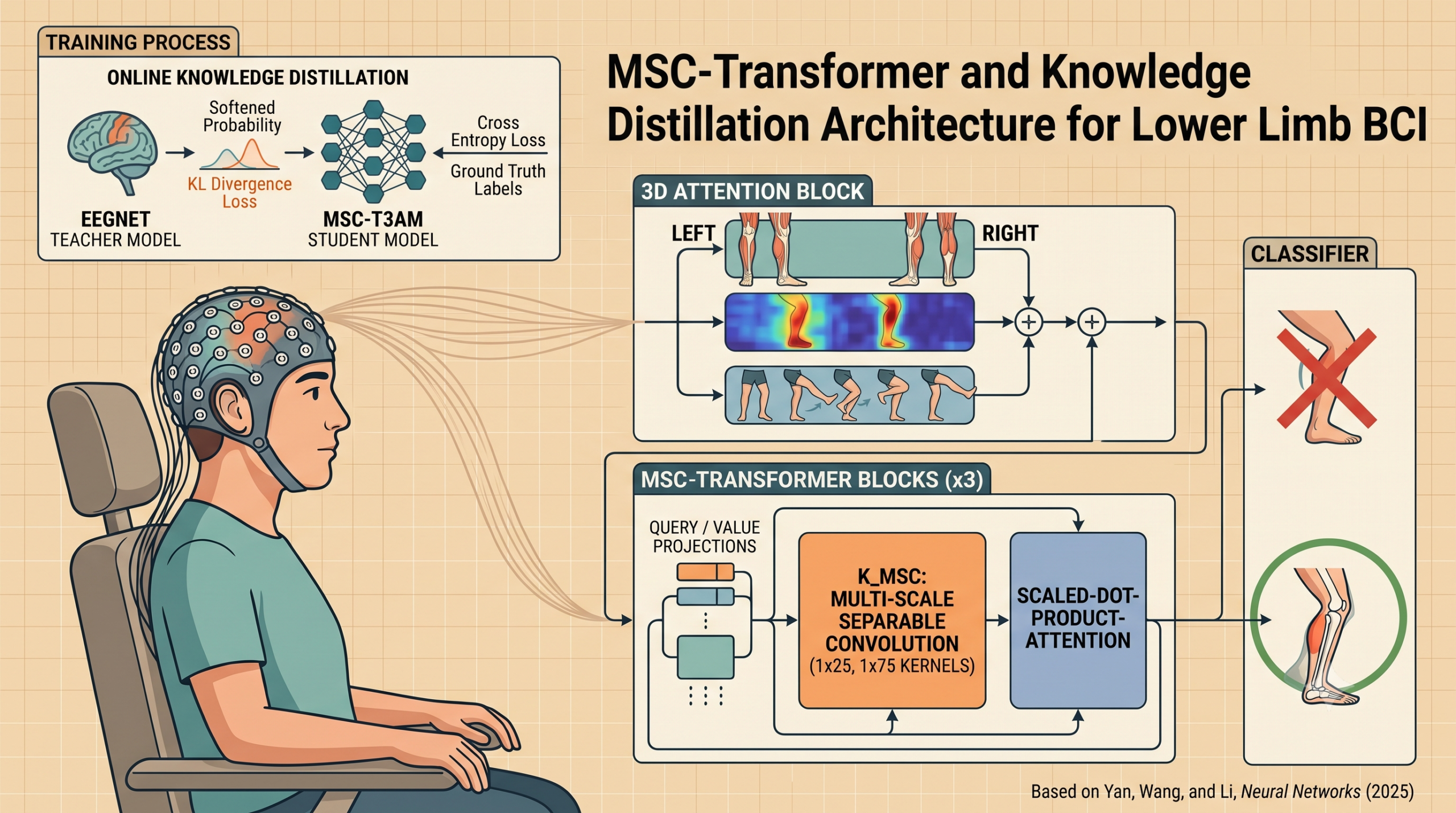
The architecture has three stages. A 3D attention block runs first, followed by three MSC Transformer blocks, followed by a plain fully connected classifier with a softmax on top. The interesting engineering sits in the first two stages.
Spatial attention, weighting the 62 channels
The raw EEG sample enters as a tensor with one filter, 62 channels, and 1500 time points. An adaptive weight tensor is multiplied against it to produce a version of the signal with F filters, still 62 channels wide. A spatial convolution then compresses the channel dimension down, and this is where the model first decides which electrodes on the scalp are worth paying attention to before anything else happens.
Filter attention, weighting which frequency band matters
After the spatial step, global average pooling collapses the signal down to one value per filter, capturing what each filter has picked up overall. A small multilayer perceptron with a reduction ratio of two then turns that into filter specific weights, effectively deciding which learned frequency filters carry the most useful information for this particular sample.
Temporal attention, weighting when in the trial it matters
The temporal path runs a point convolution to shrink the filter dimension, applies a 1 by 25 temporal convolution to catch local patterns in time, then runs another point convolution to collapse everything down to a single temporal weight per time step. The filter weight and the temporal weight are then expanded back out, added together, passed through a sigmoid, and multiplied against the original signal before being added back to it as a residual connection. That residual step matters. It means the model can lean on the reweighted features without ever fully discarding the raw signal it started with.
MSC Transformer, cutting the cost of full attention
The output of the 3D attention block feeds into three MSC Transformer blocks that are meant to capture global structure the local attention modules cannot reach. Instead of running full self attention directly on the query, key, and value projections, the model applies multi scale separable convolutions to the key projection specifically, one branch with a 1 by 25 kernel and a second branch with a 1 by 75 kernel, concatenated together before the scaled dot product attention step shown in the paper’s Figure 2. This is a fairly common trick borrowed from efficient transformer designs generally, use cheaper depthwise separable convolutions to summarize a longer sequence before the expensive attention operation runs on it, cutting compute while still exposing the model to both short range and long range temporal patterns.
That equation is the training loss for the student model under knowledge distillation, and it is worth pausing on because it is really the second half of the paper’s contribution.
Teaching the student while the teacher is still learning
Knowledge distillation trains a smaller or different shaped student model to mimic a teacher model’s output probabilities, not just the hard ground truth label. The intuition is that a teacher’s full probability distribution across all six classes, say 70 percent confidence in real movement of the right leg but also 15 percent in motor imagery of the right leg, carries information about which classes resemble each other that a single correct label throws away.
The authors picked EEGNet as the teacher, and they give three reasons in the paper. EEGNet trains quickly and reaches a useful probability distribution fast, which matters a lot for online distillation specifically. EEGNet already performs relatively well on EEG data on its own, keeping the false positive rate down so the teacher is not actively misleading the student. And EEGNet is convolutional, giving it the spatial locality bias that a pure transformer architecture lacks, so pairing a transformer student with a convolutional teacher lets the student borrow a bias it does not have natively.
There are two flavors of distillation compared here. Offline distillation pretrains the teacher fully before the student ever starts training, so the teacher is already strong from the first epoch and simply hands down fixed guidance. Online distillation trains the teacher and student at the same time, updating both every epoch, so the guidance the student receives keeps shifting as the teacher itself keeps improving.
The loss for the student combines a standard cross entropy term against the true label with a Kullback-Leibler divergence term against the softened teacher probability distribution, weighted by a coefficient alpha. A temperature parameter, set to 1.5 following prior audio synthesis work the authors cite, softens both the teacher’s and the student’s output distributions before the divergence is computed, which is the same softening trick from the original Hinton distillation paper carried over into this EEG setting.
What the numbers actually show
The dataset behind all of this comes from 28 subjects performing six lower limb actions, motor imagery, real movement, and motor observation, each split into left and right versions. Each action was repeated 72 times per subject, giving 432 trials per person in total. Recording used 62 EEG channels plus two pairs of electrooculogram channels, downsampled to 250 Hz, with a bandpass filter narrowing the usable frequency range to 8 through 30 Hz before training. Everything ran through five fold cross validation with the Adam optimizer, a 0.01 learning rate, a batch size of 16, and 200 epochs per fold.
Here is how MSC T3AM stacked up against six comparison models plus its own ablated versions, using the mean accuracy across all 28 subjects.
| Model | Mean accuracy | Standard deviation |
|---|---|---|
| EEG Conformer | 29.70% | 10.90% |
| LMDA-Net | 42.34% | 6.28% |
| FBCSP-SVM | 42.73% | 8.67% |
| DeepConvNet | 43.43% | 9.92% |
| ATCNet | 43.81% | 7.30% |
| EEGNet | 46.23% | 7.81% |
| MSC T3AM, no distillation | 47.44% | 7.03% |
| MSC T3AM, offline distillation | 47.79% | 7.37% |
| MSC T3AM, online distillation | 48.41% | 7.58% |
Two things stand out reading this table straight. First, the gap between the strongest baseline, EEGNet at 46.23 percent, and the full proposed model at 48.41 percent is real but modest, a bit over two percentage points, even though the paper’s abstract advertises an elevation of 2 to 19 percent against a few counterpart models. That headline number is technically accurate since EEG Conformer sits nearly 19 points behind, but EEG Conformer’s own accuracy of 29.70 percent with a huge 10.90 percent standard deviation looks like a model that struggled to fit this particular dataset rather than a fair ceiling for comparison. Reading the full table rather than just the top line summary gives a more grounded picture of where MSC T3AM’s real advantage sits, which is against the stronger baselines like EEGNet and ATCNet, not against the weakest one in the lineup.
Second, the six way confusion matrix reported in the paper shows imagined movement is genuinely the hard category here. Left and right motor imagery were correctly classified 36 percent and 34 percent of the time respectively, while real movement and motor observation both cleared 49 percent or higher on their strongest classes. Imagined movement was more often mistaken for real movement or observed movement than those two were mistaken for each other, which lines up with what a lot of motor imagery research already suspects, imagined movement produces a weaker and more variable cortical signature than actually moving or watching movement.
What the ablation table says versus what the paper’s text says
Here is where a close read of the paper turns up something worth flagging rather than smoothing over. The paper’s prose states plainly that removing the filter and temporal attention modules causes the biggest accuracy drop, 2.8 percentage points, followed by the MSC module at 1.2 points and spatial attention at 1 point. But Table 3 in the paper reports accuracy for every combination of modules present, and working through those combinations by comparing the full model against each three module subset gives a different ranking. Dropping spatial attention alone (leaving filter and temporal attention plus MSC) takes accuracy from 47.44 percent down to 44.62 percent, a drop of 2.82 points. Dropping filter and temporal attention alone (leaving spatial attention plus MSC) takes it to 46.29 percent, a drop of 1.15 points. Dropping MSC alone (leaving spatial plus filter and temporal attention) takes it to 46.41 percent, a drop of 1.03 points.
In other words, the raw table points to spatial attention as the module with the biggest individual contribution when removed from the full model, not filter and temporal attention as the text states. This kind of mismatch between a paper’s narrative summary and its own underlying table happens more often than readers might expect, and it is exactly the sort of detail that gets lost if an article just restates the abstract. The overall message, that all three modules add something and none of them alone explains the full gain, still holds either way. Which specific module carries the most weight is genuinely ambiguous from the published numbers, and anyone trying to reproduce or extend this work should check the authors’ code rather than trust either the abstract or the table blindly.
What the brain maps add on top of the accuracy numbers
Beyond the accuracy tables, the authors ran two visualization exercises that give a bit more confidence the model is learning something physiologically sensible rather than exploiting some quirk of the recording setup. First, they measured the Euclidean distance between the average feature vector of each of the six categories, before and after adding the MSC Transformer block, and separately before and after adding distillation. In both cases the category centers spread further apart once the full architecture and distillation were in place, which is a reasonable proxy for the categories becoming more separable in the model’s internal representation, consistent with the accuracy gains.
Second, they generated scalp topography maps from the spatial attention module’s output for two example subjects, focusing on the samples the model classified with 95 percent confidence or higher. Those maps show attention concentrated near the midline of the scalp for all six actions, with real movement trials pulling slightly more toward the frontal region and motor observation trials pulling slightly more toward the occipital region relative to imagined movement. That pattern lines up with prior findings the authors cite from fNIRS and fMRI studies of motor imagery versus real movement versus observed movement, which is a reasonable point in favor of the model picking up genuine motor cortex activity rather than an artifact.
Clinical translation gap
None of this closes the distance between a laboratory classifier and a usable clinical or assistive tool. The dataset here has 28 subjects, all presumably healthy volunteers given the trial protocol described, performing scripted actions in a controlled recording session. Patients who would actually benefit from a lower limb brain computer interface, people recovering from stroke or spinal cord injury, often have altered or degraded motor cortex signals compared to healthy volunteers, and a model trained entirely on healthy brain activity has no guarantee of transferring well to that population. The paper does not test on any clinical population, does not report cross subject generalization beyond the five fold cross validation split, and does not address the calibration time or session to session signal drift that real world BCI deployment has to handle. A five fold cross validation mean accuracy of 48.41 percent on six classes is a meaningful research result, but it sits a long way from anything that could reliably drive a rehabilitation device in real time for an individual patient today.
Clinical limitations
Worth naming directly. Twenty eight subjects is a modest sample for a six class problem, and the standard deviation across subjects, 7.58 percent for the best performing model, is large enough that individual results varied a great deal, from roughly 31 percent for the weakest subject to nearly 67 percent for the strongest. That spread suggests the model’s real world reliability would depend heavily on the individual, and any deployment would likely need per subject calibration rather than a single model applied uniformly. The paper also does not report testing across multiple recording sessions on different days, which is a known source of accuracy drop in EEG based systems generally, since electrode placement and skin conductivity shift session to session. Readers evaluating this work for anything beyond research interest should treat these as open questions the paper leaves for future work rather than issues that have already been solved.
Where this leaves the field
The honest reading of this paper is that it is a solid, carefully ablated piece of architecture and training research rather than a leap forward in absolute accuracy. Going from a 46.23 percent single best baseline to a 48.41 percent proposed model on a genuinely hard six class problem, where random guessing would land near 16.7 percent, is a real improvement worth having, and the mechanism behind it, three dimension specific attention plus a cheaper transformer plus online distillation from a fast convolutional teacher, is a reasonable and reusable recipe for other EEG classification problems beyond lower limbs specifically. The authors themselves flag two open limitations for future work, that the teacher model’s confidence in the wrong class can actively mislead the student during distillation, and that a fixed temperature parameter limits how well the distillation adapts when teacher and student probability distributions diverge sharply. Both are reasonable directions and neither is trivial to fix.
A PyTorch implementation of the architecture
The code below reconstructs the model’s architecture and training loop as described in the paper, including the 3D attention block, the multi scale separable convolution transformer blocks, and both the offline and online knowledge distillation losses. It is written to run end to end on random dummy data as a smoke test, so you can confirm every shape lines up before pointing it at real EEG.
# msc_t3am.py
# Reconstruction of MSC T3AM from Yan, Wang, and Li, Neural Networks 191 (2025) 107806
# This is an independent reimplementation for educational purposes, not the authors' original code.
import torch
import torch.nn as nn
import torch.nn.functional as F
import math


class SpatialAttention(nn.Module):
    """Channel weighted tensor plus a spatial convolution over the 62 EEG channels."""
    def __init__(self, n_channels=62, n_filters=16):
        super().__init__()
        self.adaptive_tensor = nn.Parameter(torch.randn(1, n_filters, 1, n_channels) * 0.02)
        self.spatial_conv = nn.Conv2d(n_filters, n_filters, kernel_size=(n_channels, 1), groups=n_filters)
        self.bn = nn.BatchNorm2d(n_filters)

    def forward(self, x):
        # x shape, batch by 1 by channels by time
        weighted = x * self.adaptive_tensor.transpose(2, 3)
        weighted = weighted.permute(0, 1, 3, 2)
        out = self.spatial_conv(weighted)
        out = self.bn(out)
        return F.elu(out)


class FilterAttention(nn.Module):
    """Global average pooling across the filter dimension, then an MLP for filter weights."""
    def __init__(self, n_filters, reduction=2):
        super().__init__()
        hidden = max(n_filters // reduction, 1)
        self.mlp = nn.Sequential(
            nn.Linear(n_filters, hidden),
            nn.ReLU(inplace=True),
            nn.Linear(hidden, n_filters),
        )

    def forward(self, x):
        # x shape, batch by filters by 1 by time
        pooled = x.mean(dim=3).squeeze(2)
        weight = self.mlp(pooled)
        return weight.unsqueeze(2).unsqueeze(3)


class TemporalAttention(nn.Module):
    """Point convolution, temporal convolution, point convolution to get a per time weight."""
    def __init__(self, n_filters, reduction=2):
        super().__init__()
        hidden = max(n_filters // reduction, 1)
        self.point_in = nn.Conv2d(n_filters, hidden, kernel_size=1)
        self.temporal_conv = nn.Conv2d(hidden, hidden, kernel_size=(1, 25), padding=(0, 12), groups=hidden)
        self.point_out = nn.Conv2d(hidden, 1, kernel_size=1)

    def forward(self, x):
        h = F.elu(self.point_in(x))
        h = F.elu(self.temporal_conv(h))
        weight = self.point_out(h)
        return weight


class ThreeDAttentionBlock(nn.Module):
    """Combines spatial, filter, and temporal attention with a residual connection."""
    def __init__(self, n_channels=62, n_filters=16):
        super().__init__()
        self.spatial = SpatialAttention(n_channels, n_filters)
        self.filter_attn = FilterAttention(n_filters)
        self.temporal_attn = TemporalAttention(n_filters)

    def forward(self, x):
        spatial_out = self.spatial(x)
        f_weight = self.filter_attn(spatial_out)
        t_weight = self.temporal_attn(spatial_out)
        combined = torch.sigmoid(f_weight + t_weight)
        out = spatial_out * combined + spatial_out
        return out


class MultiScaleSeparableConv(nn.Module):
    """Two branches of depthwise separable convolution at different kernel widths, concatenated."""
    def __init__(self, channels, kernel_sizes=(25, 75)):
        super().__init__()
        self.branches = nn.ModuleList([
            nn.Sequential(
                nn.Conv1d(channels, channels, kernel_size=k, padding=k // 2, groups=channels),
                nn.Conv1d(channels, channels, kernel_size=1),
            ) for k in kernel_sizes
        ])

    def forward(self, x):
        # x shape, batch by channels by sequence
        outs = [branch(x)[:, :, :x.shape[2]] for branch in self.branches]
        return torch.cat(outs, dim=1)


class MSCTransformerBlock(nn.Module):
    """Q and V get a light projection, K gets the multi scale separable convolution, then attention."""
    def __init__(self, dim, n_heads=4):
        super().__init__()
        self.dim = dim
        self.n_heads = n_heads
        self.q_proj = nn.Linear(dim, dim)
        self.v_proj = nn.Linear(dim, dim)
        self.k_msc = MultiScaleSeparableConv(dim)
        self.k_merge = nn.Linear(dim * 2, dim)
        self.out_proj = nn.Linear(dim, dim)
        self.ff = nn.Sequential(
            nn.Linear(dim, dim * 4),
            nn.GELU(),
            nn.Linear(dim * 4, dim),
        )
        self.norm1 = nn.LayerNorm(dim)
        self.norm2 = nn.LayerNorm(dim)

    def forward(self, x):
        # x shape, batch by sequence by dim
        q = self.q_proj(x)
        v = self.v_proj(x)
        k_in = x.transpose(1, 2)
        k = self.k_msc(k_in).transpose(1, 2)
        k = self.k_merge(k)

        scale = math.sqrt(self.dim)
        scores = torch.matmul(q, k.transpose(-1, -2)) / scale
        attn = F.softmax(scores, dim=-1)
        attended = torch.matmul(attn, v)
        x = self.norm1(x + self.out_proj(attended))
        x = self.norm2(x + self.ff(x))
        return x


class MSCT3AM(nn.Module):
    def __init__(self, n_channels=62, n_filters=16, n_classes=6, n_transformer_blocks=3):
        super().__init__()
        self.attention_block = ThreeDAttentionBlock(n_channels, n_filters)
        self.transformer_blocks = nn.ModuleList([
            MSCTransformerBlock(n_filters) for _ in range(n_transformer_blocks)
        ])
        self.pool = nn.AdaptiveAvgPool1d(1)
        self.classifier = nn.Linear(n_filters, n_classes)

    def forward(self, x):
        # x shape, batch by 1 by channels by time
        feats = self.attention_block(x)
        feats = feats.squeeze(2).transpose(1, 2)
        for block in self.transformer_blocks:
            feats = block(feats)
        feats = feats.transpose(1, 2)
        pooled = self.pool(feats).squeeze(-1)
        logits = self.classifier(pooled)
        return logits


def softened_log_prob(logits, temperature):
    return F.log_softmax(logits / temperature, dim=-1)


def softened_prob(logits, temperature):
    return F.softmax(logits / temperature, dim=-1)


def distillation_loss(student_logits, teacher_logits, labels, alpha=0.5, temperature=1.5):
    """Combines cross entropy against the true label with KL divergence against the teacher."""
    ce = F.cross_entropy(student_logits, labels)
    student_log_p = softened_log_prob(student_logits, temperature)
    teacher_p = softened_prob(teacher_logits.detach(), temperature)
    kl = F.kl_div(student_log_p, teacher_p, reduction="batchmean") * (temperature ** 2)
    return alpha * ce + (1 - alpha) * kl


class EEGNetTeacher(nn.Module):
    """A compact stand in for EEGNet, used as the teacher model in distillation."""
    def __init__(self, n_channels=62, n_classes=6, f1=8):
        super().__init__()
        self.temporal = nn.Conv2d(1, f1, kernel_size=(1, 64), padding=(0, 32))
        self.bn1 = nn.BatchNorm2d(f1)
        self.depthwise = nn.Conv2d(f1, f1 * 2, kernel_size=(n_channels, 1), groups=f1)
        self.bn2 = nn.BatchNorm2d(f1 * 2)
        self.pool1 = nn.AvgPool2d((1, 4))
        self.separable = nn.Conv2d(f1 * 2, f1 * 2, kernel_size=(1, 16), padding=(0, 8), groups=f1 * 2)
        self.bn3 = nn.BatchNorm2d(f1 * 2)
        self.pool2 = nn.AvgPool2d((1, 8))
        self.classifier = nn.LazyLinear(n_classes)

    def forward(self, x):
        h = F.elu(self.bn1(self.temporal(x)))
        h = F.elu(self.bn2(self.depthwise(h)))
        h = self.pool1(h)
        h = F.elu(self.bn3(self.separable(h)))
        h = self.pool2(h)
        h = h.flatten(1)
        return self.classifier(h)


def train_step_online(student, teacher, optimizer_s, optimizer_t, x, y, alpha=0.5, temperature=1.5):
    """One step of online knowledge distillation, teacher and student both update."""
    teacher_logits = teacher(x)
    teacher_ce = F.cross_entropy(teacher_logits, y)
    optimizer_t.zero_grad()
    teacher_ce.backward()
    optimizer_t.step()

    student_logits = student(x)
    loss = distillation_loss(student_logits, teacher_logits.detach(), y, alpha, temperature)
    optimizer_s.zero_grad()
    loss.backward()
    optimizer_s.step()
    return loss.item()


def evaluate(model, x, y):
    model.eval()
    with torch.no_grad():
        logits = model(x)
        preds = logits.argmax(dim=-1)
        acc = (preds == y).float().mean().item()
    model.train()
    return acc


if __name__ == "__main__":
    # Smoke test on dummy data shaped like the paper's setup,
    # 62 channels, 1500 time points, six classes, small batch.
    torch.manual_seed(0)
    batch_size, n_channels, n_time, n_classes = 8, 62, 1500, 6
    dummy_x = torch.randn(batch_size, 1, n_channels, n_time)
    dummy_y = torch.randint(0, n_classes, (batch_size,))

    student = MSCT3AM(n_channels=n_channels, n_filters=16, n_classes=n_classes)
    teacher = EEGNetTeacher(n_channels=n_channels, n_classes=n_classes)

    optimizer_s = torch.optim.Adam(student.parameters(), lr=0.01)
    optimizer_t = torch.optim.Adam(teacher.parameters(), lr=0.01)

    for epoch in range(3):
        loss_value = train_step_online(student, teacher, optimizer_s, optimizer_t, dummy_x, dummy_y)
        acc = evaluate(student, dummy_x, dummy_y)
        print(f"epoch {epoch} loss {loss_value:.4f} dummy accuracy {acc:.4f}")

    print("Smoke test complete, shapes and gradients flow end to end.")
Conclusion
The core achievement here is a workable answer to a question the field had mostly left alone, whether EEG carries enough separable signal to tell left lower limb activity apart from right lower limb activity across three very different behavioral conditions, imagined, real, and observed movement. Forty eight percent mean accuracy on a six class problem where chance sits near seventeen percent is not a headline grabbing number, but it is a genuine, statistically tested improvement over every convolutional and prior attention based baseline the authors tried, and it comes with an unusually thorough ablation study that lets a reader see exactly which pieces of the architecture are doing the work, even where that ablation study contradicts the paper’s own summary of it.
The conceptual shift worth carrying forward is treating filter, spatial, and temporal information as three separate problems rather than one blended attention computation. That is not a lower limb specific idea, and there is nothing in the architecture that would stop someone from applying the same three way attention split to upper limb motor imagery, to sleep stage classification, or to any other EEG task where frequency content, scalp location, and timing all carry genuinely different kinds of information. The knowledge distillation piece is similarly transferable, and the finding that online distillation edged out offline distillation, even by a modest margin, is a useful data point for anyone deciding how to pair a fast convolutional teacher with a heavier transformer student in their own EEG pipeline.
What the paper does not settle, and is honest enough to say so itself, is how a fixed distillation temperature holds up when a teacher and student diverge more sharply than they did here, and what happens when the teacher’s own confidence works against the student rather than for it. Both are reasonable next steps, and neither requires a fundamentally new architecture to test, just a more adversarial training setup than the one reported here.
The honest remaining limitation, stated plainly rather than buried, is that everything in this paper was tested on healthy volunteers in a single recording session, which is a meaningful distance from the patients who would actually benefit from a lower limb brain computer interface in a rehabilitation setting. Sample size, cross session stability, and clinical population testing are all open questions the authors leave for future work rather than problems they claim to have solved.
None of that undercuts the value of the engineering here. Attention mechanisms tuned to the actual structure of a signal, rather than applied generically, keep proving out across EEG research, and pairing a strong classifier with a genuinely knowledgeable teacher through distillation is a reasonably cheap way to squeeze out real gains without a much bigger model. For a subfield that has spent most of its energy on hands, a serious attempt at separating left and right legs across three behavioral conditions is a step worth building on, and the code being public means the next person to test that fixed temperature limitation does not have to start from zero.
Honest limitations
Beyond the clinical limitations already covered above, a few methodological points are worth naming plainly. The study used a single hardware setup, one NVIDIA GTX 1050 Ti, and a fixed learning rate of 0.01 across all compared models, which is a reasonable choice for a fair comparison but does mean none of the baseline models were individually tuned to their own best hyperparameters, so the gap between MSC T3AM and, say, ATCNet or LMDA-Net could shift under a more exhaustive tuning pass for each competitor. The five fold cross validation scheme also mixes trials from the same subjects across folds rather than testing on entirely held out subjects, based on how the accuracy table is organized by subject with per subject means, which means the reported numbers reflect within subject generalization more than across subject generalization, an important distinction for anyone thinking about deploying a single trained model across a new patient population.
Frequently asked questions
What does MSC T3AM stand for
Multi scale separable convolutional transformer based filter spatial temporal attention model. The name describes its three main ingredients, multi scale separable convolutions inside the transformer blocks, and a three dimensional attention block covering filter, spatial, and temporal structure in the EEG signal.
How accurate is the model at classifying lower limb EEG
The full model with online knowledge distillation reached a mean accuracy of 48.41 percent across 28 subjects on a six class task, left and right versions of motor imagery, real movement, and motor observation. Chance performance on six classes is roughly 16.7 percent.
What is the difference between online and offline knowledge distillation in this paper
Offline distillation pretrains the teacher model, EEGNet in this case, completely before training the student. Online distillation trains the teacher and student together at the same time, updating both every epoch. The paper found online distillation performed slightly better, 48.41 percent mean accuracy against 47.79 percent for offline.
Which category was hardest for the model to classify correctly
Motor imagery, meaning imagined movement without any actual muscle activity, was the hardest category. It was more often confused with real movement or motor observation than those two categories were confused with each other, based on the confusion matrix reported in the paper.
Is this technology ready for use in stroke rehabilitation or assistive devices
No. The study was conducted on 28 healthy volunteers under laboratory conditions in a single recording session. It does not test on any clinical population, does not evaluate performance across multiple days, and does not address the calibration or signal drift issues that a real deployment would face. This is research grade work, not a clinical tool.
Where can I read the original paper and get the code
The paper is published in Neural Networks, volume 191, 2025, article 107806, and the authors’ code is available on their linked GitHub repository referenced in the paper itself.
Read the full paper for the complete equations, the additional visualization figures, and the full per subject accuracy table.
Read the paper View the codeThis analysis is based on the published paper and an independent evaluation of its claims.