
Key points
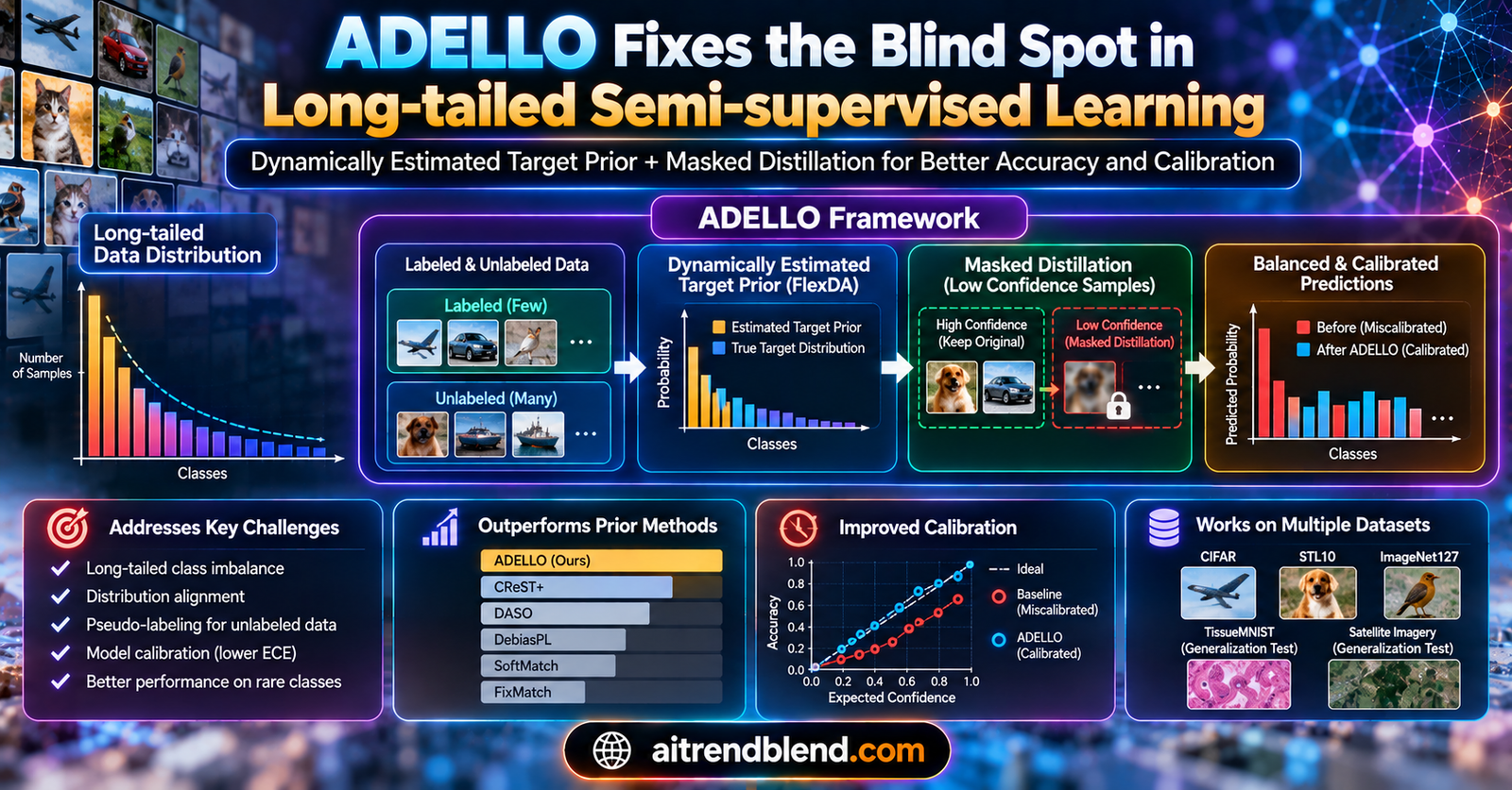
- ADELLO, short for Align and Distill Everything All at Once, is a semi-supervised learning framework built to handle long-tailed, imbalanced classification when the labeled and unlabeled data do not share the same class distribution.
- Its core component, Flexible Distribution Alignment or FlexDA, dynamically estimates the unknown unlabeled class distribution during training and gradually steers the classifier from that estimate toward a fully balanced one by the end of training.
- A second component, complementary consistency regularization, rescues the unlabeled samples a standard confidence threshold would normally throw away, using a temperature scaled distillation loss instead of hard pseudo-labels.
- Across CIFAR10-LT, CIFAR100-LT, STL10-LT, and the naturally imbalanced ImageNet127 benchmark, ADELLO ranked first overall by Friedman ranking against eight competing methods, while also cutting expected calibration error roughly in half on the hardest STL10-LT setting.
- ADELLO is not the single best method in every individual benchmark cell tested, and the paper is upfront that all of its long-tailed benchmarks still assume every class is known in advance, a limitation the authors name directly rather than gloss over.
The problem with training on whatever data you can actually get
Semi-supervised learning exists to solve a specific, very common headache, that labeling data is expensive, so you want to train mostly on a small labeled set plus a much larger pool of unlabeled data. The standard playbook, popularized by a method called FixMatch, is straightforward. Feed the model a weakly augmented version of an unlabeled image, and if the model’s confidence on its own prediction clears a threshold, treat that prediction as a pseudo-label and train the model to reproduce it on a more heavily, strongly augmented version of the same image. It works well in tidy, balanced benchmark settings.
Real datasets are rarely tidy. The paper opens with the observation that class distributions in the wild tend to be long-tailed, a few frequent classes dominating a long list of rare ones, and that this alone biases a classifier toward the frequent, head classes even before semi-supervised learning enters the picture. Layer pseudo-labeling on top of that imbalance and the problem compounds, since a model that is already biased toward head classes will generate pseudo-labels that are also biased toward head classes, which then get fed right back into training as if they were ground truth. The result, as the authors put it, is imbalanced pseudo-label distributions that further neglect rare classes, and probabilities that are poorly calibrated, meaning the model’s stated confidence stops meaning much of anything.
The harder wrinkle, and the one the paper spends most of its effort on, is that the labeled data’s class distribution and the unlabeled data’s class distribution frequently do not match at all. A small labeled set might happen to have relatively more examples of some rare class purely by chance of who bothered to label what, while the much larger unlabeled pool follows a genuinely different, and generally unknown, distribution. The paper calls this mismatch label distribution shift, and it breaks a quiet assumption baked into most prior distribution alignment methods, that the labeled prior is a decent stand in for the unlabeled prior.
What earlier fixes assumed, and where they fell short
Distribution alignment, the general strategy of correcting a model’s pseudo-label distribution to better match a target prior, is not a new idea. ReMixMatch used an exponential moving average of predictions to align pseudo-labels toward the labeled prior in balanced settings. CReST+ extended a similar pseudo-label correction into long-tailed settings, using a multi-generational training schedule. Logit adjustment methods correct a fully supervised model’s bias toward a uniform target directly inside the loss function rather than by touching pseudo-labels. DebiasPL and UDAL each combine pseudo-label correction with an adjusted unsupervised loss, with UDAL specifically adding a progressive schedule that smooths the target prior over the course of training.
| Method | Correction strategy | Target prior it assumes | Progressive over training |
|---|---|---|---|
| ReMixMatch | Pseudo-label adjustment | Long-tailed labeled prior | No |
| CReST+ | Pseudo-label adjustment | Long-tailed labeled prior | Yes |
| Logit adjustment | Supervised loss adjustment | Uniform | No |
| DebiasPL | Pseudo-label plus unsupervised loss | Uniform | No |
| UDAL | Supervised and unsupervised losses | Long-tailed labeled prior | Yes |
| ADELLO, the paper’s method | Supervised and unsupervised losses | Adaptive, estimated from unlabeled data | Yes |
Notice the pattern across almost every prior row, the target prior each method aligns toward is fixed in advance, either matching the long-tailed labeled distribution or assuming a uniform distribution outright. Every one of those choices silently assumes the labeled prior is a reasonable stand in for whatever the unlabeled data actually looks like. ADELLO is the only row in that table whose target prior is adaptive, estimated directly and continuously from the unlabeled data itself rather than assumed in advance.
The Bayes-optimal reasoning behind FlexDA
The paper grounds its design in a short chain of statistical reasoning that is worth walking through slowly, because it explains why FlexDA needs three different notions of what a good classifier is, at three different points in training, rather than just one.
Start by assuming an early training phase produces a scorer that has perfectly fit the labeled distribution, meaning its output is proportional to the labeled posterior. Under a specific, common assumption called label shift, where the underlying likelihood of what an image looks like given its true class stays the same across the labeled and unlabeled data, but the class priors themselves differ, there is a clean way to correct that labeled scorer into a version optimized for the unlabeled data instead, simply by rescaling it with the ratio of the unlabeled prior to the labeled prior. That adjusted scorer turns out to be the Bayes-optimal choice for generating correct pseudo-labels on the unlabeled data specifically.
But generating good pseudo-labels during training is not actually the end goal. At inference time, the goal is a classifier that treats every class fairly, minimizing what is called the balanced error rate, a metric that by design does not favor whichever classes happened to be more common in training or test data. That requires one more rescaling step, adjusting the unlabeled-optimized scorer again, this time toward a uniform prior where every class is equally likely.
The scorer trained on labeled data, \( g_L(x) \), is rescaled by the ratio between the unknown unlabeled prior \( Q(y) \) and the labeled prior \( P_L(y) \), producing a scorer proportional to the unlabeled posterior, the Bayes-optimal target for pseudo-labeling.
A second rescaling, this time by the ratio between a uniform prior \( P_{bal}(y) = 1/K \) across all \( K \) classes and the unlabeled prior, turns the pseudo-labeling-optimized scorer into a fully balanced one, proportional to the balanced posterior that minimizes the balanced error rate at inference time.
The catch, which the paper is direct about, is that the unlabeled prior \( Q(y) \) needed for both of these corrections is unknown in practice, and even the labeled prior can be a poor, noisy estimate of the truth when only a handful of labeled examples exist per class. FlexDA’s entire design exists to work around not knowing \( Q(y) \) exactly, by estimating it continuously from the model’s own behavior on unlabeled data as training proceeds.
How FlexDA actually adjusts the loss
FlexDA tracks a running estimate of the unlabeled prior, \( \hat{Q}(y) \), using an exponential moving average of the model’s own soft predictions on weakly augmented unlabeled images throughout training. That estimate then feeds into a smoothed, time-varying target prior that starts out close to the estimated unlabeled distribution and is gradually pulled toward a uniform, balanced distribution as training proceeds.
A schedule controls how quickly the target prior transitions from matching the estimated unlabeled distribution toward the balanced one, where \( t \) is the current training step, \( t_{total} \) is the total number of steps, \( d \) controls the schedule’s speed, and \( \alpha_{min} \) sets the minimum residual bias still allowed at the end of training. When \( \alpha_t \) is near one early in training, the target prior closely tracks the estimated unlabeled distribution. As \( \alpha_t \) decays toward \( \alpha_{min} \), the target prior smooths toward uniform.
That schedule feeds directly into two logit-adjusted loss terms, one for the labeled data and one for the unlabeled consistency loss, both built on the same underlying trick, adding a correction term inside the softmax before computing cross entropy, a technique known as logit adjustment.
The supervised loss adjusts the model’s raw logits on labeled data by the log ratio of the labeled prior to the current smoothed target prior, nudging the classifier away from simply reproducing the labeled data’s own bias.
The consistency loss on confidently pseudo-labeled unlabeled data applies a matching correction, using the ratio between the estimated unlabeled prior and the current smoothed target, restricted to samples whose confidence mask \( \mathcal{M}(u_b) \) clears the threshold.
The net effect, as the paper walks through statistically, is that early in training the adjusted classifier behaves close to the Bayes-optimal pseudo-labeling scorer for the unlabeled data specifically, and by the end of training, as the target prior smooths fully to uniform, the same adjusted classifier converges toward the balanced scorer that minimizes balanced error rate at inference. One loss structure, two different optimality targets, stitched together by a single decaying schedule.
Rescuing the unlabeled data a confidence threshold would normally discard
A standard confidence threshold, set at 0.95 in this paper following FixMatch’s own convention, throws away every unlabeled sample the model is not extremely confident about. Early in training, and especially for rare tail classes the model has barely seen, that means discarding a large share of available unlabeled data, precisely the data that might have helped the most. Making matters worse, the paper notes that FlexDA’s own progressive debiasing can itself reduce pseudo-label confidence as training proceeds, further shrinking the pool of samples the standard consistency loss is allowed to use.
The authors’ answer is complementary consistency regularization, a masked distillation loss that specifically targets the samples the confidence threshold rejects, using the complementary mask, one minus the standard confidence mask, to isolate exactly the low-confidence samples that would otherwise contribute nothing to training.
Rather than assigning a hard, one class pseudo-label to these low-confidence samples, this loss uses temperature-scaled soft predictions, \( p^{1/T}(y|x) = \sigma(\frac{1}{T}f(x)) \), as a softer distillation target, applied only to samples the complementary mask \( \mathcal{M}^{C}(u_b) \) selects.
A deliberate design choice sets this apart from several prior methods the authors cite. Some earlier approaches sharpen, meaning use a low temperature on, these low-confidence predictions, which the authors argue increases the risk of confirmation bias, essentially trusting an uncertain guess more strongly than its actual reliability warrants. ADELLO does the opposite, using a higher temperature, softer distillation for exactly the samples it is least sure about.
Rather than hand tuning a temperature for every dataset, ADELLO infers it automatically from how far the estimated unlabeled prior has drifted from a uniform distribution, measured by KL divergence. A near-balanced unlabeled distribution produces a temperature near one, encouraging more confident distillation, while a heavily imbalanced distribution produces a higher temperature, encouraging more cautious, softer distillation. This value is computed once after a brief warm-up period and then held fixed for the rest of training.
What got tested, and on what
The experiments span four main benchmark families. CIFAR10-LT and CIFAR100-LT are long-tailed versions of the standard CIFAR datasets, built by sampling class sizes according to a controllable imbalance ratio, tested under two separate label budgets equal to one third and one ninth of the total available data. STL10-LT downsamples the labeled portion of STL10 and pairs it with an extra 100,000 unlabeled images that deliberately include out-of-distribution classes drawn from the broader ImageNet taxonomy, a genuinely harder and more realistic test since not every unlabeled image even belongs to a known class. ImageNet127 is the most demanding test of all, a naturally, not artificially, imbalanced dataset with roughly a 286 to 1 imbalance ratio built by grouping the full 1,000 ImageNet classes into 127 categories, evaluated with only 10 percent of the data labeled.
Every configuration used FixMatch as its underlying semi-supervised backbone with the standard 0.95 confidence threshold, Wide-ResNet-28-2 for the CIFAR and STL10 experiments and ResNet-50 for ImageNet127, with results averaged across three independent runs and reported as the mean test balanced accuracy over the final 20 training epochs. To fairly compare methods across many different experimental settings at once, the authors use Friedman ranking, a statistical method for aggregating a method’s relative rank across multiple conditions into one overall score, rather than relying on any single benchmark number to declare a winner.
Where ADELLO actually won, and where it did not
Under controlled label shift, where the researchers deliberately varied how different the unlabeled class distribution was from the labeled one across forward, balanced, and reversed long-tailed settings, ADELLO achieved the best overall Friedman rank across all six CIFAR10-LT and CIFAR100-LT conditions tested, ahead of DARP, CReST+, ABC, DASO, DebiasPL, CoSSL, UDAL, and SoftMatch. It is worth being precise about what that ranking does and does not mean. ADELLO was not the single highest scoring method in every individual cell, CoSSL edged it out on the CIFAR10-LT forward setting at 84.6 percent against ADELLO’s 83.8 percent, CReST+ won the CIFAR10-LT balanced setting at 92.6 percent against ADELLO’s 91.9 percent, and ABC won the CIFAR10-LT reversed setting at 87.0 percent against ADELLO’s 86.1 percent. What earned ADELLO the top overall rank was consistency, it never fell far behind the leader in any single setting while dominating outright across every CIFAR100-LT condition, and no other method matched that same combination of consistently strong performance across every tested scenario.
Under limited labeled data conditions, ADELLO again took the top Friedman rank across CIFAR10-LT, CIFAR100-LT, and STL10-LT. The STL10-LT result stands out specifically because of the out-of-distribution unlabeled data baked into that benchmark. At an imbalance ratio of 20, ADELLO reached 74.6 percent accuracy, a gain the paper reports as roughly 8 percentage points over CoSSL and, at an imbalance ratio of 10, roughly 4.5 percentage points over ABC. The authors offer a specific explanation for the gap, that a strong competing baseline, SoftMatch, mistakenly classifies out-of-distribution data as one of the known classes using confident hard pseudo-labels, while ADELLO’s complementary consistency component instead predicts soft pseudo-labels for exactly this kind of ambiguous data, a more appropriate response to genuinely unfamiliar input.
On ImageNet127, tested at both 32 by 32 and 64 by 64 pixel resolution, ADELLO posted the best balanced accuracy outright at both resolutions, 47.5 percent and 58.0 percent respectively, ahead of the next best method CoSSL by 3.8 and 4.2 percentage points, and ahead of the strongest UDAL configuration by 3.4 and 5.7 percentage points. Because ImageNet127’s imbalance occurs naturally rather than being synthetically constructed, this result is a meaningful signal that the method’s benefits are not an artifact of how the synthetic CIFAR-based benchmarks happen to be built.
The calibration story is arguably the bigger finding
Accuracy tables are the usual headline in papers like this, but the calibration results are where ADELLO’s advantage becomes genuinely dramatic rather than incremental. Expected calibration error measures the gap between a model’s stated confidence and its actual accuracy, and a well calibrated model that says it is 90 percent confident should, in practice, be right about 90 percent of the time.
| Method | CIFAR10-LT100 | STL10-LT20 | CIFAR100-LT50, forward |
|---|---|---|---|
| FixMatch | 23.9 | 37.8 | 37.4 |
| DARP | 19.2 | 31.6 | 33.3 |
| ABC | 13.5 | 24.6 | 24.5 |
| CoSSL | 12.1 | 22.7 | 31.2 |
| UDAL | 12.9 | 25.7 | 31.1 |
| ADELLO, the paper’s method | 10.4 | 6.9 | 26.1 |
Expected calibration error, where lower is better, drops to single digits for ADELLO on STL10-LT20, a stark contrast against every competing method still sitting in the 20s or higher. That result earned ADELLO the top overall Friedman rank for both expected calibration error and the related, worse case oriented maximum calibration error metric across every dataset tested. The authors tie this directly to the same out-of-distribution robustness seen in the accuracy results, attributing the improvement specifically to the combination of flexible distribution alignment with complementary consistency regularization, rather than either piece alone.
Significantly, the key to enhanced calibration in LTSSL contexts lies not just in the naive distillation of all samples, but in the strategic combination of soft pseudo-labels for underconfident samples and hard pseudo-labels for those with high confidence. From the paper’s ablation discussion, explaining why masked distillation specifically, not distillation in general, drives the calibration gain
What the ablation studies actually isolate
The paper’s ablation experiments are unusually careful about separating what each component contributes to accuracy versus calibration, and the two stories diverge in an interesting way. On CIFAR100-LT50 across three imbalance ratios, adding FlexDA alone to the FixMatch baseline produced accuracy gains of 4.2, 5.0, and 5.8 percentage points. Adding complementary consistency regularization alone produced smaller gains. Combining both produced the largest jump, 4.8, 8.9, and 7.6 percentage points over FlexDA alone at the three imbalance ratios tested. Interestingly, a variant that distilled all samples indiscriminately, rather than masking to just the low-confidence ones, achieved accuracy roughly comparable to the full masked version, and even slightly ahead of it in the balanced case, but the masked version won more consistently under severe imbalance.
On calibration specifically, that comparison flips more decisively in favor of masking. The full FlexDA plus complementary consistency combination achieved an expected calibration error of 6.9 percent on STL10-LT20, while the indiscriminate distillation variant only reached 10.0 percent, a meaningfully larger gap than the two showed on accuracy. This is the clearest evidence in the paper that masking specifically, targeting distillation only at samples the model is genuinely unsure about, rather than distillation as a general technique, is what drives the calibration benefit.
Two smaller hyperparameter studies round out the picture. The progressive scheduler’s speed, controlled by the parameter \( d \), performed best at a moderate setting between 1 and 3, while an aggressive, instant debiasing schedule at \( d = 0 \) actively hurt performance, confirming that the gradual transition itself, not just the final balanced target, matters. The minimum residual bias parameter, \( \alpha_{min} \), showed the model was not especially sensitive to its exact value, performing best near zero but only degrading modestly even at less ideal settings. Separately, the inferred, automatically computed temperature from the KL divergence formula performed nearly as well as manually tuning a custom temperature for every dataset, a meaningful practical convenience for anyone trying to apply this method without extensive per-dataset tuning.
The efficiency detail easy to miss
A detail buried in the paper’s appendix deserves more attention than it usually gets in coverage of methods like this. ADELLO’s total training time on CIFAR100-LT50, run on a single Nvidia V100 GPU, was 5 hours and 18 minutes, closely matching FixMatch’s 5 hours 15 minutes and ABC’s 5 hours 21 minutes. Several competing methods took substantially longer, CReST+ at 6 hours 22 minutes, CoSSL at 7 hours 29 minutes, DARP at 7 hours 43 minutes, and DASO at 19 hours 32 minutes, nearly four times ADELLO’s runtime. The authors attribute ADELLO’s efficiency to a deliberate design constraint, avoiding extra forward passes, auxiliary classifier networks, or data resampling schemes that several competing methods rely on. A method that wins on both accuracy and calibration while adding negligible training overhead is a considerably more practical proposition than one that wins on accuracy alone at several times the compute cost.
A brief note on the cross domain generalization test
Beyond its main natural image benchmarks, the paper includes a smaller appendix experiment testing whether the same approach transfers to image domains quite different from ordinary photographs. Using the same CIFAR10-LT style protocol and hyperparameters, the authors built long-tailed versions of TissueMNIST, a set of small greyscale microscopy images across 8 tissue classes, and EuroSAT, a set of small satellite imagery patches across 10 land use classes. ADELLO outperformed FixMatch, DARP, DebiasPL, and UDAL on both, reaching 52.3 to 54.4 percent accuracy across different label shift settings on the microscopy dataset and 94.1 percent on the satellite dataset. It is worth being precise about what this experiment shows and does not show, it is a general tissue type classification benchmark used here purely to test whether the method generalizes across visual domains, not a diagnostic task, and the paper draws no clinical conclusions from it.
Honest limitations
The authors name their most significant limitation directly rather than leaving a reader to infer it. Every long-tailed semi-supervised benchmark the paper is aware of operates under what is called the closed-world assumption, meaning every class that will ever appear is already known and labeled in advance. Real world deployment rarely offers that guarantee. The STL10-LT results, where genuinely out-of-distribution unlabeled data is present, offer a partial, encouraging signal that ADELLO handles unfamiliar data more gracefully than its competitors, but the authors are careful to frame this as suggestive promise rather than a solved problem, since STL10-LT’s out-of-distribution classes still come from a known, related taxonomy rather than being truly arbitrary or adversarial.
The paper is also explicit that its framework was developed and tested exclusively for classification, and that extending the same distribution alignment ideas to more complex vision tasks such as object detection, instance segmentation, or tracking remains unexplored future work rather than a demonstrated capability. Beyond what the authors state directly, a careful reader should also note that ADELLO’s advantage, while consistent across the Friedman rankings, is not universal in every single reported comparison, several individual benchmark cells were won by other methods, and the overall ranking system, while a reasonable and standard way to aggregate performance across many conditions, can obscure exactly how close or how large any single head to head gap actually was. All reported results also come from a single hardware setup, a lone Nvidia V100 GPU, and three independent runs per configuration, a reasonably standard but not exhaustive number of repetitions for establishing how much of any given gap reflects a genuine, repeatable effect versus ordinary training variance.
Conclusion
What makes this paper worth understanding beyond its benchmark tables is the clarity of its underlying argument. Long-tailed semi-supervised learning has a genuine, well defined statistical target, a classifier that behaves one way during pseudo-label generation and a subtly different way at final inference, and most prior work either ignored that distinction or assumed away the harder half of the problem, the possibility that unlabeled data simply does not look like labeled data. FlexDA’s contribution is less a clever trick than a disciplined follow through on that statistical reasoning, estimating what needs to be estimated, adjusting what the Bayes-optimal math says should be adjusted, and doing so on a schedule rather than all at once.
The complementary consistency piece is the paper’s second, quieter insight, that a fixed confidence threshold designed to prevent a model from trusting its own bad guesses also, as an unavoidable side effect, throws away a disproportionate share of exactly the data that would help correct those guesses fastest, the data belonging to classes the model has barely learned yet. Rescuing that discarded data through soft, temperature scaled distillation rather than treating it as ordinary hard pseudo-labels is a genuinely different choice than simply lowering the confidence threshold, and the ablation results make a reasonably convincing case that this specific choice, not distillation in general, is what drives the calibration gains in particular.
The calibration results deserve more attention than a typical accuracy focused reading of this paper would give them. A classifier that is merely more accurate on average is a narrower kind of progress than a classifier that is both more accurate and honest about when it does not know something, and the gap ADELLO opens up on expected calibration error, especially on the benchmark containing genuinely unfamiliar unlabeled data, is large enough to suggest the two properties, accuracy and calibration, were not being optimized together nearly as well by prior long-tailed semi-supervised methods.
None of this closes the gap to open-world deployment, and the authors do not pretend otherwise. A closed, known set of classes, a classification only scope, and a modest number of repeated runs on a single GPU setup are all real, stated boundaries on what this paper demonstrates. What it demonstrates within those boundaries is unusually well reasoned, a method whose design choices trace back cleanly to an explicit statistical argument, tested honestly enough that the paper’s own tables show it losing individual comparisons here and there rather than sweeping every benchmark outright.
For anyone building a real classifier on real, messy, unevenly labeled data, the transferable lesson here is less about ADELLO specifically and more about the two questions its design insists on asking separately, whether your model’s confidence can be trusted, and whether the data you are training on actually resembles the data you plan to deploy against. Most systems only manage to be honest about one of those two questions at a time. This paper argues, with reasonably convincing evidence, that treating them as one connected problem produces a genuinely better answer to both.
Reference implementation of the core losses in PyTorch
The following is an original, simplified, runnable PyTorch implementation inspired by the FlexDA logit-adjusted losses, the progressive scheduler, and the complementary consistency regularization described in the paper. It is a compact educational reconstruction of the core loss mechanics, not the authors’ own code, built to illustrate the approach on dummy data with a working smoke test.
# adello_flexda_core.py
# Educational reimplementation of the FlexDA logit-adjusted supervised
# and consistency losses, the progressive alpha_t scheduler, and the
# complementary consistency regularization loss, inspired by "Flexible
# Distribution Alignment: Towards Long-tailed Semi-supervised Learning
# with Proper Calibration", arXiv:2306.04621.

import torch
import torch.nn.functional as F

NUM_CLASSES = 10
CONFIDENCE_THRESHOLD = 0.95
EMA_MOMENTUM = 0.999


class FlexDAState:
    """Tracks the running estimate of the unlabeled prior Q_hat and the
    progressive scheduler alpha_t, following Section 4.1."""
    def __init__(self, num_classes, labeled_prior, d=2, alpha_min=0.1):
        self.num_classes = num_classes
        self.labeled_prior = labeled_prior  # P_L(y), fixed from labeled data counts
        self.q_hat = torch.full((num_classes,), 1.0 / num_classes)  # starts uniform
        self.d = d
        self.alpha_min = alpha_min

    def update_q_hat(self, weak_probs_unlabeled):
        """EMA update of Q_hat using the batch mean of weakly augmented
        unlabeled predictions, following Table 1's use of an EMA."""
        batch_mean = weak_probs_unlabeled.mean(dim=0)
        self.q_hat = EMA_MOMENTUM * self.q_hat + (1 - EMA_MOMENTUM) * batch_mean

    def alpha_t(self, step, total_steps):
        """Implements the alpha_t schedule that smooths the target prior
        from the estimated unlabeled prior toward a balanced one."""
        progress = min(step / max(total_steps, 1), 1.0)
        return 1.0 - (1.0 - self.alpha_min) * (progress ** self.d)

    def target_prior(self, step, total_steps, eps=1e-8):
        """Computes the smoothed target prior Q_hat_alpha_t used inside
        both FlexDA loss terms."""
        a_t = self.alpha_t(step, total_steps)
        powered = (self.q_hat + eps) ** a_t
        return powered / powered.sum()

    def inferred_temperature(self, balanced_prior, eps=1e-8):
        """Implements Eq. 7, T = exp(KL(P_bal || Q_hat))."""
        kl = (balanced_prior * (balanced_prior / (self.q_hat + eps) + eps).log()).sum()
        return torch.exp(kl).clamp(min=1.0)


def flexda_supervised_loss(logits_labeled, y_labeled, labeled_prior, target_prior, eps=1e-8):
    """Implements Eq. 4, the logit-adjusted supervised loss."""
    correction = torch.log((labeled_prior + eps) / (target_prior + eps))
    adjusted_logits = logits_labeled + correction
    return F.cross_entropy(adjusted_logits, y_labeled)


def flexda_consistency_loss(logits_strong_unlabeled, probs_weak_unlabeled, q_hat, target_prior, threshold=CONFIDENCE_THRESHOLD, eps=1e-8):
    """Implements Eq. 5, the logit-adjusted unsupervised consistency loss,
    restricted to confidently pseudo-labeled samples."""
    confidence, pseudo_label = probs_weak_unlabeled.max(dim=1)
    mask = (confidence >= threshold).float()

    correction = torch.log((q_hat + eps) / (target_prior + eps))
    adjusted_logits = logits_strong_unlabeled + correction
    per_sample_loss = F.cross_entropy(adjusted_logits, pseudo_label, reduction="none")

    if mask.sum() == 0:
        return torch.tensor(0.0), mask
    return (per_sample_loss * mask).sum() / mask.sum(), mask


def complementary_consistency_loss(logits_weak_unlabeled, logits_strong_unlabeled, confidence_mask, q_hat, target_prior, temperature, eps=1e-8):
    """Implements Eq. 6 combined with the FlexDA bias correction, the
    complementary consistency loss applied only to low-confidence,
    complementary-masked samples, using soft, temperature-scaled
    targets rather than hard pseudo-labels."""
    complementary_mask = 1.0 - confidence_mask
    if complementary_mask.sum() == 0:
        return torch.tensor(0.0)

    soft_target_weak = F.softmax(logits_weak_unlabeled / temperature, dim=1)
    correction = torch.log((q_hat + eps) / (target_prior + eps))
    adjusted_strong_logits = (logits_strong_unlabeled + correction) / temperature
    log_soft_strong = F.log_softmax(adjusted_strong_logits, dim=1)

    per_sample_kl = F.kl_div(log_soft_strong, soft_target_weak, reduction="none").sum(dim=1)
    return (per_sample_kl * complementary_mask).sum() / complementary_mask.sum()


def smoke_test():
    """Runs one training step on random dummy data to confirm every
    loss term and the scheduler state are wired together correctly."""
    torch.manual_seed(0)
    labeled_prior = F.softmax(torch.linspace(2, -2, NUM_CLASSES), dim=0)  # a synthetic long-tailed prior
    balanced_prior = torch.full((NUM_CLASSES,), 1.0 / NUM_CLASSES)
    state = FlexDAState(NUM_CLASSES, labeled_prior, d=2, alpha_min=0.1)

    batch = 16
    logits_labeled = torch.randn(batch, NUM_CLASSES, requires_grad=True)
    y_labeled = torch.randint(0, NUM_CLASSES, (batch,))
    logits_weak_unlabeled = torch.randn(batch, NUM_CLASSES, requires_grad=True)
    logits_strong_unlabeled = torch.randn(batch, NUM_CLASSES, requires_grad=True)

    probs_weak = F.softmax(logits_weak_unlabeled, dim=1)
    state.update_q_hat(probs_weak.detach())

    step, total_steps = 50_000, 262_144
    target_prior = state.target_prior(step, total_steps)
    temperature = state.inferred_temperature(balanced_prior)

    l_s = flexda_supervised_loss(logits_labeled, y_labeled, labeled_prior, target_prior)
    l_u, mask = flexda_consistency_loss(logits_strong_unlabeled, probs_weak.detach(), state.q_hat, target_prior)
    l_uc = complementary_consistency_loss(logits_weak_unlabeled.detach(), logits_strong_unlabeled, mask, state.q_hat, target_prior, temperature)

    total_loss = l_s + l_u + l_uc
    total_loss.backward()

    print("alpha_t at this step", round(state.alpha_t(step, total_steps), 4))
    print("Inferred temperature", round(float(temperature), 4))
    print("Supervised loss", round(float(l_s), 4))
    print("Consistency loss", round(float(l_u), 4))
    print("Complementary consistency loss", round(float(l_uc), 4))
    print("Smoke test completed without errors")


if __name__ == "__main__":
    smoke_test()
Frequently asked questions
What does long-tailed semi-supervised learning actually mean
It describes training a classifier on a small labeled dataset plus a larger unlabeled dataset, where the classes involved are imbalanced, meaning a few classes have many examples and most classes have far fewer, following what is called a long-tailed distribution. The added complication addressed in this paper is that the labeled data’s class distribution and the unlabeled data’s class distribution frequently do not match each other, and the unlabeled distribution is usually unknown in advance.
What is distribution alignment and why does it need to be flexible
Distribution alignment is a technique that corrects a model’s pseudo-label predictions to better match some target class distribution rather than letting the model drift toward whichever classes it happens to predict most confidently. Most prior distribution alignment methods assumed a fixed target prior, either matching the labeled data’s own distribution or a uniform distribution. FlexDA is flexible because it dynamically estimates the actual, otherwise unknown unlabeled class distribution during training and gradually shifts its target from that estimate toward a balanced one, rather than assuming either extreme from the start.
What is model calibration and why does the paper care about it so much
Model calibration measures whether a model’s stated confidence matches its actual accuracy, so a well calibrated model that says it is 90 percent confident about a prediction should be correct about 90 percent of the time. The paper found that class imbalance and mismatched labeled and unlabeled data distributions tend to produce poorly calibrated, overconfident models, and that ADELLO substantially reduced this calibration error compared to every other method tested, particularly on a benchmark containing unlabeled data from classes not seen in the labeled set.
Does ADELLO win every single benchmark it was tested on
No, and the paper’s own tables show this plainly. ADELLO achieved the best overall rank when performance was aggregated across every tested condition using a statistical method called Friedman ranking, but in several individual comparisons other methods scored higher, including CoSSL on one CIFAR10-LT setting and CReST+ and ABC on two others. ADELLO’s advantage comes from performing consistently well across a wide range of conditions rather than dominating every single one.
Was this method tested on medical images
A brief appendix experiment tested the method on TissueMNIST, a small greyscale microscopy image dataset with 8 general tissue type classes, alongside a separate satellite imagery dataset, specifically to check whether the approach generalizes across different visual domains beyond ordinary photographs. This was a general classification generalization test, not a diagnostic evaluation, and the paper does not make any clinical claims based on this result.
What is the main limitation the authors acknowledge
The authors state directly that every long-tailed semi-supervised learning benchmark they are aware of, including the ones used in this paper, assumes a closed world where every class that will appear is already known and labeled in advance. They also note the framework was developed and tested only for classification, leaving tasks like object detection, instance segmentation, or tracking as unexplored future work.
Read the original research
This analysis is based on the paper posted to arXiv, with a version dated 15 July 2024.
Pingback: 7 Powerful Reasons BAST-Mamba Is Revolutionizing Binaural Sound Localization — Despite the Challenges - aitrendblend.com