
- Knowledge distillation
- Temperature softmax
- KL divergence
- Soft targets
- Decoupled KD
- Feature distillation
- PyTorch
An engineer has a network that scores well on the validation set and a latency budget it misses by a factor of ten. She trains a model a tenth the size on the same labels and loses accuracy she cannot afford. Then she trains that same small model on the big one’s predicted probabilities, and a surprising share of the lost accuracy comes back.
Nothing about the images changed. Only the targets did. Why a vector of probabilities teaches better than a label is a question with a precise mathematical answer, and it turns out to have several layers. This piece works through them one derivation at a time.
Key points
- Temperature divides logits before the softmax, which compresses log odds and exposes how the teacher ranks the wrong classes.
- The soft target gradient is \( (q_i – p_i)/T \), and at high temperature it shrinks as \( 1/T^2 \). That is where the famous \( T^2 \) factor comes from.
- In the high temperature limit the Hinton loss becomes plain mean squared error between centered logits, so logit matching is a special case.
- Near agreement, KL divergence is a quadratic form weighted by the teacher’s Fisher matrix, which explains why low temperatures ignore very unlikely classes.
- Soft labels keep the expected loss but cut its variance, and at T equal to 1 distillation is label smoothing with a learned, per example smoothing distribution.
- A runnable PyTorch file at the end checks every identity in the article numerically.
Why a Teacher’s Wrong Answers Are Worth Copying
The idea is older than most people assume. In 2006, Cristian Bucilă, Rich Caruana and Alexandru Niculescu-Mizil showed that a large ensemble could be compressed into a single network by labeling a big pool of synthetic data with the ensemble and training the small model on those labels. Their paper, simply titled Model Compression, framed the teacher as a function to be approximated rather than a set of answers to be copied.
Eight years later Jimmy Ba and Rich Caruana pushed the point further in Do Deep Nets Really Need to be Deep? They trained shallow networks to regress the logits of deep ones with a squared error loss, and the shallow students got much closer to their deep teachers than shallow networks trained on labels alone. The target was the raw logit vector, before any softmax.
Then in 2015 Geoffrey Hinton, Oriol Vinyals and Jeff Dean published Distilling the Knowledge in a Neural Network, the paper that named the field. They kept the softmax, added a temperature, and gave practitioners a loss they could drop into any classifier. They also offered an intuition that stuck. A picture of a BMW has only a tiny chance of being mistaken for a garbage truck, yet that mistake is still far more likely than mistaking it for a carrot. On MNIST, one handwritten 2 might get a probability of one in a million of being a 3 and one in a billion of being a 7, while another 2 gets the reverse. The label says 2 in both cases. The probabilities say which kind of 2 it is.
That relative information about wrong classes is what later writers called dark knowledge. The rest of this article is about how the math extracts it, why it helps, and where it stops helping. If you want the wider context of how this fits alongside pruning and quantization, the knowledge distillation and model compression hub collects every related analysis on the site.
Temperature Is a Knob on Log Odds
Write the teacher’s logits for one input as \( v \in \mathbb{R}^K \) and the student’s as \( z \in \mathbb{R}^K \). The tempered softmax turns logits into probabilities.
The cleanest way to see what T does is to look at a ratio of two probabilities. The normalizer cancels and only the logit gap is left.
So temperature does one thing. It divides every log odds ratio by the same constant. A gap of 8.5 nats between two classes becomes a gap of about 2.1 nats at T equal to 4. Rankings never change, only the contrast.
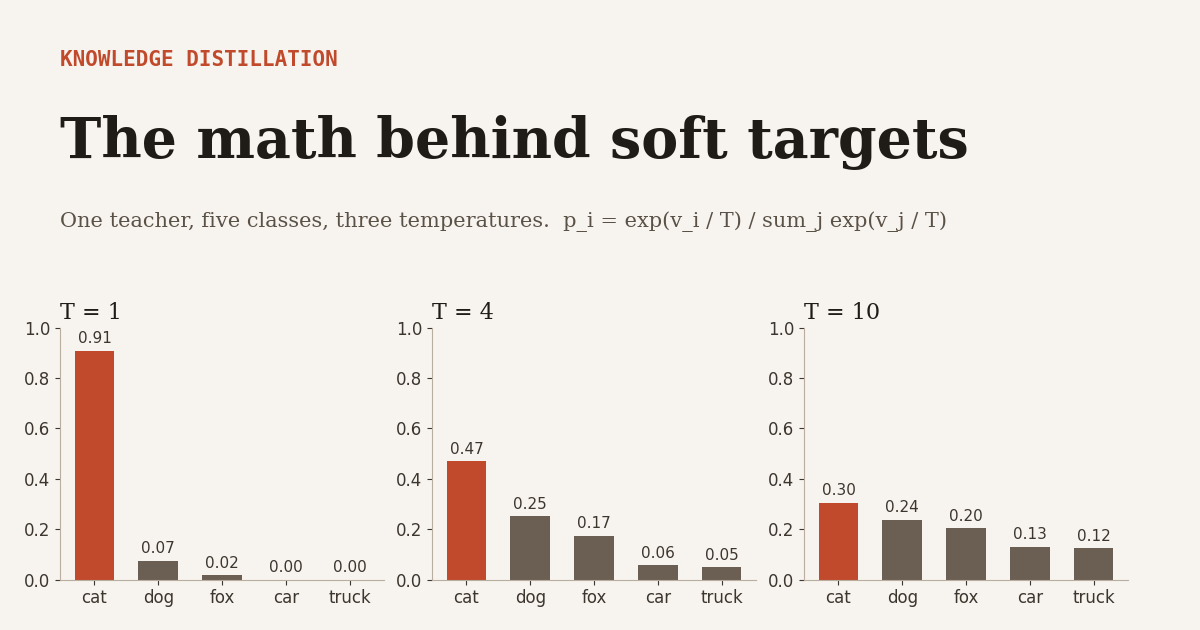
A concrete case makes this less abstract. Suppose a teacher looks at a photo of a cat and produces logits of 9.0 for cat, 6.5 for dog, 5.0 for fox, 0.5 for car and 0.0 for truck. Here is what the student would be asked to match.
| Temperature | cat | dog | fox | car | truck | Entropy (bits) | dog to car ratio |
|---|---|---|---|---|---|---|---|
| T = 1 | 0.908 | 0.075 | 0.017 | 0.0002 | 0.0001 | 0.51 | 403 |
| T = 4 | 0.470 | 0.252 | 0.173 | 0.056 | 0.050 | 1.90 | 4.5 |
| T = 10 | 0.305 | 0.237 | 0.204 | 0.130 | 0.124 | 2.24 | 1.8 |
Computed by aitrendblend for the illustrative logits above. The maximum possible entropy for five classes is about 2.32 bits.
At T equal to 1 the teacher is almost a one hot label. The fact that a car is a worse guess than a fox is buried in the fourth decimal place, and a cross entropy loss will barely notice it. At T equal to 4 the same fact is plainly visible. At T equal to 10 it is still there, but the distribution is drifting toward uniform and the signal that cat is the right answer is starting to fade.
That tension between exposing structure and washing it out is the whole temperature story in miniature. The rest of the math explains exactly how each choice changes what the student learns.
The Loss Hinton Wrote Down
The standard objective mixes two terms. One is ordinary cross entropy with the true label at temperature 1. The other asks the student’s tempered distribution to match the teacher’s.
The weight \( \alpha \) sets how much the student listens to the teacher versus the label. The \( T^2 \) looks like a fudge factor. It is not, and deriving it is the best way to understand the gradient.
Before that, one small identity. KL divergence is cross entropy minus entropy.
The teacher is frozen, so its entropy is a constant with respect to the student’s parameters. Minimizing KL and minimizing cross entropy against soft targets produce identical gradients. The KL form is preferred in code only because its value reaches zero when the student matches perfectly, which makes the number easier to read in a training log.
The classic response based distillation pipeline. Only the student receives gradients. Diagram by aitrendblend.
Following the Gradient Through the Softmax
Take the soft cross entropy \( C = -\sum_j p_j \log q_j \), dropping the superscript T for readability. The derivative of a log softmax output with respect to a logit is a classic result.
Plug it into the loss and use the fact that teacher probabilities sum to one.
This is the same shape as the familiar gradient of ordinary cross entropy, student probability minus target, with one extra factor of \( 1/T \). Hinton and colleagues derive exactly this expression in section 2.1 of their paper. Each logit gets pushed in proportion to how much the student over or under predicts that class relative to the teacher.
Look back at the table. At T equal to 1, the car entry of the teacher is 0.0002. Whatever the student predicts for car, the gradient on the car logit is tiny because both probabilities are close to zero. At T equal to 4, the teacher asks for 0.056 on car, and a student that has pushed car down to nothing now receives a real correction.
Where the T squared comes from
Now let the temperature grow. For large T every exponent is small, so a first order expansion \( e^{x} \approx 1 + x \) is accurate.
Softmax does not change when a constant is added to every logit, so without loss of generality both logit vectors can be centered to have zero mean. The sums in the denominators vanish and the gradient collapses to something very simple.
There it is. The soft target gradient scales as \( 1/T^2 \). If you raise the temperature from 2 to 8 without compensating, the soft term’s pull on the student drops by a factor of 16 while the hard label term stays exactly where it was. The \( \alpha \) you tuned at one temperature would mean something completely different at another. Multiplying the soft loss by \( T^2 \) cancels this and keeps the balance between the two terms roughly fixed as you sweep T. Hinton, Vinyals and Dean make exactly this point in the paper.
The limit is logit matching
Equation 8 is the gradient of a familiar loss. Multiply the soft term by \( T^2 \), as Equation 3 does, and the result is the gradient of a squared error between centered logits.
This is the Ba and Caruana objective, up to centering and a constant. So their logit regression and Hinton’s tempered KL are not rival methods. One is the limit of the other. The PyTorch file at the end confirms Equation 9 numerically at T equal to 1000, where the two losses agree to better than one percent.
The limit also explains a practical observation in the original paper. When the student is much too small to absorb everything the teacher knows, intermediate temperatures work better than very high ones. At infinite temperature every logit error counts equally, including errors on hugely negative logits that carry little useful meaning. A finite temperature quietly discounts those, as the next section shows.
A Geometric Reading, KL as a Weighted Distance on Logits
The high temperature limit is one end of a spectrum. What happens in between becomes clear from a second order expansion of KL around the point where student and teacher agree. Write \( \delta = (z – v)/T \) for the scaled logit gap and \( p \) for the teacher’s tempered distribution.
The matrix \( \Sigma_p \) is the covariance of a one hot draw from the teacher’s distribution, and it is also the Fisher information of the softmax in logit coordinates. Its diagonal entries are \( p_i(1 – p_i) \). That gives a very direct reading of what the loss cares about. The error on logit i is weighted by roughly how uncertain the teacher is about class i.
Return to the cat example. At T equal to 1 the diagonal weights for cat, dog, fox, car and truck are about 0.083, 0.069, 0.016, 0.0002 and 0.0001. An error on the car logit costs several hundred times less than the same error on the dog logit. The student is effectively told to get the top three classes right and ignore the rest. At T equal to 4 the weights become 0.249, 0.188, 0.143, 0.053 and 0.047, so car and truck now count for roughly a quarter as much as dog. At very high temperature all weights approach \( 1/K \) and the metric turns Euclidean, which is Equation 9 again.
Temperature, then, is not just a softening trick. It chooses the metric in which student and teacher logits are compared. Low temperatures give a sharply weighted metric that focuses on the plausible classes. High temperatures give a flat metric that treats every class the same. That is a much more useful mental model when tuning than the vague idea of making targets softer.
Every temperature defines a different distance between logit vectors. Small T asks the student to match the teacher only on classes the teacher finds plausible. Large T asks it to match every logit equally. A small student with limited capacity usually benefits from a middle setting that spends its effort where the teacher’s knowledge is reliable.
Why Soft Labels Reduce Variance
The gradient story explains how distillation transfers information. It does not explain why a student trained on soft targets often generalizes better than the same student trained on the true labels. A statistical argument, developed carefully by Aditya Krishna Menon and colleagues at Google in A Statistical Perspective on Distillation at ICML 2021, fills that gap.
Imagine an oracle teacher that outputs the true class probabilities \( p^{*}(x) = \Pr(y \mid x) \). Cross entropy is linear in its target, so taking the expectation over the random label gives the same answer as plugging in the oracle’s probabilities.
Both targets therefore aim at the same population risk. The difference is noise. By the law of total variance, the per example loss with a sampled label has variance equal to the variance of its conditional mean plus the average conditional variance. The soft target keeps only the first piece.
Lower variance in the empirical risk means the minimizer of the training loss sits closer to the minimizer of the true risk for a given sample size. In a toy simulation in the code below, with three classes and random class probabilities, the variance of the per example loss fell from about 0.77 with sampled labels to about 0.25 with the true probabilities, while the mean stayed the same.
A real teacher is not an oracle. Menon and colleagues show that the benefit depends on how close the teacher’s probabilities are to the true ones, which trades the variance reduction against a bias term. That is one reason calibration matters for teachers, and one reason a very accurate but overconfident teacher can distill poorly. The Hinton paper offers a vivid data point on the variance effect. A speech model trained on only 3 percent of the data with hard labels reached 44.5 percent test frame accuracy and overfit badly, while the same model trained on soft targets, produced by a model trained on the full training set, reached 57.0 percent, close to the 58.9 percent of a baseline trained on everything.
When the distilled model is much too small to capture all of the knowledge in the cumbersome model, intermediate temperatures work best.Hinton, Vinyals and Dean, 2015
At temperature 1, distillation is learned label smoothing
Set T to 1 in Equation 3 and use the fact that cross entropy is linear in its first argument. The two terms merge into one.
Label smoothing is the special case where \( p \) is the uniform distribution. Distillation replaces that uniform smear with a distribution that is different for every example and shaped by learned similarity between classes. Li Yuan and colleagues pushed this connection in Revisiting Knowledge Distillation via Label Smoothing Regularization, arguing that much of the benefit of distillation is regularization and showing that even poorly trained teachers can help.
The connection runs the other way too. Rafael Müller, Simon Kornblith and Geoffrey Hinton found in When Does Label Smoothing Help? that teachers trained with label smoothing make worse teachers. Smoothing pulls penultimate layer representations into tight, evenly spaced class clusters, and that erases the relative similarity information in the logits that distillation needs. Put in the language of this article, a smoothed teacher’s \( \Sigma_p \) has lost exactly the off target structure that the student was supposed to learn.
Splitting the Loss in Two, Decoupled Knowledge Distillation
The KL term hides a coupling that Borui Zhao and colleagues made explicit in Decoupled Knowledge Distillation at CVPR 2022. Let t be the index of the true class. Group the teacher’s distribution into a binary part \( b^{p} = (p_t,\, 1 – p_t) \) and a renormalized distribution over the other classes, \( \hat{p}_i = p_i / (1 – p_t) \) for \( i \ne t \). Do the same for the student.
Split the KL sum into the true class and the rest, substitute \( p_i = (1-p_t)\hat{p}_i \) and \( q_i = (1-q_t)\hat{q}_i \) in the second part, and the log of a product separates into a sum.
The first term, target class distillation, only transfers how confident the teacher is about the right answer, which the authors interpret as the difficulty of the example. The second term, non target class distillation, carries the ranking among the wrong classes, which is the dark knowledge proper.
The coupling is the factor \( 1 – p_t \). On the examples where the teacher is most confident, the very examples where it is most likely to be right, the non target term is multiplied by something close to zero. The better the teacher, the more its dark knowledge is suppressed. Zhao and colleagues concluded that the non target term is the main reason logit distillation works and proposed weighting the two parts independently, \( \alpha\,\mathrm{TCKD} + \beta\,\mathrm{NCKD} \), with \( \beta \) usually much larger than \( \alpha \). The code below checks Equation 14 to machine precision on random logits.
This is a good example of why the math pays off. The coupling was sitting inside the Hinton loss for seven years, and it only becomes visible when you write the KL term out and regroup it.
Beyond Logits, Matching Features and Relations
Logits are a narrow channel. A penultimate layer with 512 dimensions compressed into ten class scores throws away a great deal of what the teacher knows. A second family of methods distills intermediate representations directly.
Hints and attention maps
Adriana Romero and colleagues introduced FitNets in 2015, where a thin but deep student learns to reproduce a teacher’s intermediate feature map through a small learned regressor \( r \) that bridges the dimension mismatch.
Sergey Zagoruyko and Nikos Komodakis proposed a lighter alternative in their attention transfer work. Instead of matching full feature tensors, collapse the channel axis into a spatial map that shows where the network is looking, normalize it, and match those maps.
Because the channel dimension is summed away, attention transfer needs no regressor, which removes a source of instability and a set of extra parameters.
Relations between examples
Wonpyo Park and colleagues argued in Relational Knowledge Distillation that the geometry of a batch may matter more than any single embedding. Their distance loss normalizes pairwise distances by their mean \( \mu \) and matches them with a Huber loss \( \ell_{\delta} \), so the student can live in a different space, even one of different dimension, as long as it preserves the teacher’s relative distances.
Yonglong Tian, Dilip Krishnan and Phillip Isola took the information theoretic route in Contrastive Representation Distillation. Their objective maximizes a lower bound on the mutual information between teacher and student representations. The InfoNCE form of such a bound treats distillation as a matching problem, where the student must pick out the teacher embedding of the same input from a set of N candidates.
The appeal here is that KL on softmax outputs treats each output dimension separately, while a contrastive objective captures dependencies across the whole representation. CRD itself uses a large memory bank of negatives. The implementation below uses in batch negatives, a simpler variant with a weaker bound because N is just the batch size.
| Family | What is matched | Typical loss | Extra modules | Main weakness |
|---|---|---|---|---|
| Response (Hinton KD) | Tempered class probabilities | \( T^2 \) scaled KL | None | Only K numbers per example |
| Logit regression | Centered logits | Mean squared error | None | Weights meaningless negative logits fully |
| Decoupled KD | Target and non target parts separately | \( \alpha \) TCKD plus \( \beta \) NCKD | None | Two weights to tune |
| FitNets hint | Intermediate feature maps | Squared error after regressor | Regressor | Sensitive to layer choice |
| Attention transfer | Normalized spatial attention | Squared error on maps | None | Discards channel information |
| Relational KD | Pairwise distances in a batch | Huber loss | None | Depends on batch composition |
| Contrastive (CRD) | Joint representation structure | InfoNCE style bound | Two projection heads, memory bank | Needs many negatives |
Summary by aitrendblend. Methods are frequently combined, with a response loss as the base and one feature loss on top.
Many recent systems covered on this site mix these families. DAIT inserts an adaptive intermediate teacher between CLIP and a small classifier, which is a capacity gap fix in disguise. CD-FKD distills features across weather domains for detection. TabKD shows the same principles in a data free setting for tabular models, where the student never sees real training data at all.
What Theory Says About When It Works
A clean, general theorem that predicts when distillation helps does not yet exist. What exists is a set of partial results that each explain one part of the picture.
Linear models and privileged information
Mary Phuong and Christoph Lampert studied linear and deep linear classifiers in Towards Understanding Knowledge Distillation at ICML 2019. In that setting they could bound how fast the student’s risk falls with the number of transfer examples, and they traced the speed to three factors. The geometry of the data, the bias of gradient descent toward particular solutions, and a property they called strong monotonicity, meaning the student’s risk always goes down as the training set grows. It is a narrow setting, but it is one of the few where the benefit of soft targets can be proven rather than observed.
David Lopez-Paz and colleagues, working with Léon Bottou, Bernhard Schölkopf and Vladimir Vapnik, connected distillation to learning using privileged information in Unifying Distillation and Privileged Information. In Vapnik’s framework a teacher that has access to extra information at training time can, under some conditions, speed up the rate at which a student learns. Distillation becomes a special case where the extra information is simply the output of a stronger model.
The capacity gap as a projection problem
Jang Hyun Cho and Bharath Hariharan reported in On the Efficacy of Knowledge Distillation that larger, more accurate teachers often do not make better teachers, and that stopping the teacher’s training early can help. Seyed Iman Mirzadeh and colleagues proposed a teacher assistant, a medium sized network that sits between a large teacher and a small student.
The math gives a compact way to see why. If the student family is \( \mathcal{Q} \), distillation searches for the member closest to the teacher in forward KL.
This is what information geometers call a moment projection, and it is mass covering. The student is penalized heavily wherever the teacher puts probability and the student does not. If the teacher’s function is far outside what the student can represent, the projection spends its capacity trying to cover details it cannot reach, and the leftover error can be large. An early stopped teacher or an assistant is a nearer target, so less is wasted. Framing it this way also suggests the diagnostic to run. Measure the student’s KL to the teacher on held out data, not just its accuracy.
Self distillation and the regularization view
Distillation still helps when teacher and student share the same architecture. Tommaso Furlanello and colleagues showed in Born Again Neural Networks that a student identical to its teacher can outperform it. Hossein Mobahi, Mehrdad Farajtabar and Peter Bartlett gave a mechanism in a study of self distillation in Hilbert space. For kernel regression, each round of self distillation progressively shrinks the set of basis functions the solution can use. The first few rounds reduce overfitting. Too many rounds cause underfitting. Self distillation, in their analysis, is a regularizer whose strength grows with every round.
Zeyuan Allen-Zhu and Yuanzhi Li offered a different account for deep networks in their theory of ensembles and distillation. When data has a multi view structure, where each class can be recognized from several distinct features, individual networks each latch onto a subset of those features. An ensemble collects more of them, and distillation passes that broader coverage into a single model through the soft targets. The site’s analysis of GATES and self distillation in language models shows how these ideas are being adapted to generative settings.
Forward and reverse KL for generative students
Everything above uses forward KL, teacher first. For language models that generate long sequences, some work switches the order. Yuxian Gu and colleagues argued in MiniLLM that reverse KL is a better fit for small generative students.
Forward KL punishes the student for missing any mode of the teacher, which pushes a small model to spread thin across outputs it cannot generate well. Reverse KL punishes the student for putting mass where the teacher has none, which makes it mode seeking. It is content to cover a few of the teacher’s modes well. Rishabh Agarwal and colleagues added a second fix in generalized knowledge distillation, training the student on sequences it generates itself so the training distribution matches what it will see at inference. The same projection logic from Equation 19 applies, only the direction of the divergence changes what kind of approximation error the student accepts.
Diffusion models have their own branch of this story, where the student learns to reproduce many denoising steps in one. The site’s piece on implicit generator matching for one step diffusion covers a recent example.
Distillation works through at least three separate mechanisms. It transfers class similarity structure, it reduces the variance of the training loss, and it regularizes. Which one dominates depends on the teacher’s calibration, the capacity gap, and how much data the student sees. Diagnosing which mechanism you rely on tells you what to tune.
What the Original Experiments Actually Showed
For all its theoretical afterlife, the 2015 paper made its case with two compact experiments. The numbers are worth having in front of you, since they are often quoted loosely.
| Setting | Model | Result reported |
|---|---|---|
| MNIST | Large net, two hidden layers of 1200 units, strong regularization | 67 test errors |
| MNIST | Small net, two hidden layers of 800 units, no regularization | 146 test errors |
| MNIST | Same small net trained on soft targets at T = 20 | 74 test errors |
| MNIST, no 3s in transfer set | Distilled net, after raising the bias for class 3 by 3.5 | 109 errors, 14 of them on the 1010 test 3s |
| Speech acoustic model | Baseline single model | 58.9% frame accuracy, 10.9% WER |
| Speech acoustic model | Ensemble of 10 models | 61.1% frame accuracy, 10.7% WER |
| Speech acoustic model | Single model distilled from the ensemble | 60.8% frame accuracy, 10.7% WER |
Figures as reported by Hinton, Vinyals and Dean (2015), arXiv:1503.02531. WER is word error rate.
The row with no 3s in the transfer set is the most striking result in the paper and the most direct evidence for dark knowledge. The student never saw a single example of the digit 3 during distillation. It learned what a 3 looks like entirely from how the teacher’s probability for class 3 rose and fell on images of other digits. Once its bias for that class was corrected, it recognized 98.6 percent of the test 3s. No label can carry that kind of information. Only the relative probabilities can.
The speech result is the practical one. The distilled single model recovered 1.9 of the 2.2 points of frame accuracy the ensemble gained over the baseline, and matched the ensemble’s word error rate, at a tenth of the inference cost.
A Practical Recipe Grounded in the Math
The derivations above translate into a short set of defaults that most practitioners converge on after some trial and error.
Start with the classic loss of Equation 3 and always keep the \( T^2 \) factor, or your \( \alpha \) will silently change meaning every time you touch the temperature. A temperature between 2 and 8 is a reasonable first sweep, and smaller students usually want the lower end, for exactly the reason Equation 10 gives. Their capacity is better spent on the plausible classes than on matching logits the teacher itself considers irrelevant.
Set \( \alpha \) high, often 0.7 to 0.9, when the teacher is strong and well calibrated. Lower it when the teacher is overconfident or when its accuracy is close to the student’s. If the teacher was trained with label smoothing, expect weaker transfer and consider a teacher trained without it.
When the capacity gap is large, try an earlier teacher checkpoint or an intermediate model before reaching for a more complicated loss. If response distillation plateaus, add one feature level loss, typically attention transfer for convolutional networks because it needs no regressor, and weight it so its gradient magnitude is comparable to the response term. Decoupled KD is worth trying whenever the teacher is very confident on most training examples, because that is exactly the regime where the \( 1 – p_t \) coupling hurts.
Finally, track two numbers during training, the student’s accuracy and its agreement with the teacher on held out data. They tell you different things, as the next section explains. For a broader view of how distillation interacts with other compression tools, the site’s analysis of why pruning before training can improve generalization is a useful companion read.
Limitations and Open Questions
The most uncomfortable finding in recent years came from Samuel Stanton, Pavel Izmailov, Polina Kirichenko, Alexander Alemi and Andrew Gordon Wilson in Does Knowledge Distillation Really Work? at NeurIPS 2021. They separated two goals that are usually blurred together. Generalization asks whether the student does well on test data. Fidelity asks whether the student actually reproduces the teacher’s predictions. They found that students often match their teachers poorly, even in cases where the student has enough capacity to match them, and they traced much of the gap to optimization difficulty rather than to capacity. Distillation often works, but frequently not for the reason its name suggests.
That finding sits awkwardly next to the clean derivations above. The gradient of Equation 6 says the student is pulled toward the teacher. In practice it is pulled, but it does not arrive. The variance and regularization arguments may explain more of the observed benefit than faithful imitation does.
The theory has other gaps. The strongest guarantees, those of Phuong and Lampert and of Mobahi and colleagues, hold for linear models or kernel regression. Deep network results rely on structural assumptions about the data, such as the multi view setting, that are hard to verify on a real dataset. Nobody has a formula that takes a teacher, a student and a dataset and returns the best temperature.
Distillation also copies what it should not. A teacher’s biases, spurious correlations and miscalibration are all part of its output distribution, and the student inherits them along with the useful structure. The mass covering property of forward KL makes this worse, since the student is penalized for ignoring anything the teacher believes.
And the costs are real. Training the teacher, running it over the full training set, and tuning T, \( \alpha \) and any feature loss weights can take more compute than training the student alone many times over. For small projects, a well regularized student trained on labels is sometimes the more sensible choice.
Conclusion
Strip away the vocabulary and knowledge distillation is a change of target. Instead of asking a small network to predict a label, we ask it to predict a distribution produced by a larger one. Everything else follows from the math of that substitution. The tempered softmax rescales log odds. The gradient is the difference between two probability vectors divided by T. The \( T^2 \) factor is what keeps that gradient comparable across temperatures, and the high temperature limit turns the whole thing into logit regression.
The conceptual shift is in how to think about temperature. It is tempting to treat T as a softening knob. The second order expansion shows it is better understood as a choice of metric. Low temperatures compare student and teacher only on the classes the teacher finds plausible. High temperatures compare them everywhere. That single reframing explains why intermediate temperatures suit small students, why logit matching sometimes overfits noise in very negative logits, and why decoupling the target and non target terms can help confident teachers.
The same machinery transfers well beyond image classification. Variance reduction applies to any loss that is linear in its target. The projection view of Equation 19 explains capacity gaps in speech, language and detection alike. Swapping forward KL for reverse KL, as in generative language model distillation, is a change in which approximation errors the student is allowed to make. Feature and relational losses carry the idea into settings where there are no class probabilities at all.
What remains unresolved is why distillation works as well as it does given how imperfectly students actually imitate their teachers. The fidelity results suggest that a meaningful share of the benefit is regularization and variance reduction rather than knowledge transfer in the literal sense. Theory that covers realistic deep networks, and practical rules for picking temperature and weights without a grid search, are both still open problems.
The best place to start is still the three line derivation of Equation 6. Once you see that the student is being pushed by the difference between two probability vectors, and that temperature decides which entries of those vectors are large enough to matter, most of the design choices in modern distillation start to look less like tricks and more like consequences.
Complete PyTorch Implementation
The file below is an independent educational reimplementation written by aitrendblend, not official code from any of the papers cited. It implements the classic loss, logit matching, decoupled KD, a FitNets hint, attention transfer, a relational distance loss and an in batch contrastive loss, then trains a small student from a larger teacher on dummy data. The final block runs numerical checks of Equations 6, 9, 10, 12, 13 and 14. On a CPU the whole script finishes in under a minute, and every check prints True.
"""
Knowledge distillation, the math in runnable form.
Independent educational implementation by aitrendblend. Not official code from any paper.

Contents
  1. Temperature softmax and the classic Hinton et al. (2015) KD loss with the T^2 factor
  2. Logit matching (Ba and Caruana, 2014) and the high temperature limit check
  3. Decoupled KD (Zhao et al., 2022) with an exact decomposition check
  4. Feature losses: FitNets hint, attention transfer, relational distance, contrastive (InfoNCE style)
  5. Teacher and student CNNs, training loop, evaluation, and a smoke test on dummy data
  6. Numerical checks of every identity derived in the article
"""
import math
import torch
import torch.nn as nn
import torch.nn.functional as F

torch.manual_seed(0)


# ---------------------------------------------------------------------------
# 1. Temperature softmax and the classic KD objective
# ---------------------------------------------------------------------------
def soft_probs(logits: torch.Tensor, T: float) -> torch.Tensor:
    """p_i = exp(z_i / T) / sum_j exp(z_j / T)"""
    return F.softmax(logits / T, dim=-1)


def kd_loss(student_logits, teacher_logits, T: float = 4.0) -> torch.Tensor:
    """T^2 * KL(p_teacher^T || q_student^T), averaged over the batch.

    The T^2 factor keeps gradient magnitudes comparable to the hard label term,
    because d KL / d z scales as 1/T^2 at high temperature.
    """
    log_q = F.log_softmax(student_logits / T, dim=-1)
    p = F.softmax(teacher_logits / T, dim=-1)
    return F.kl_div(log_q, p, reduction="batchmean") * (T * T)


def hinton_objective(student_logits, teacher_logits, targets, T=4.0, alpha=0.9):
    """(1 - alpha) * CE(y, q^1) + alpha * T^2 * KL(p^T || q^T)"""
    hard = F.cross_entropy(student_logits, targets)
    soft = kd_loss(student_logits, teacher_logits, T)
    return (1.0 - alpha) * hard + alpha * soft


# ---------------------------------------------------------------------------
# 2. Logit matching, the T -> infinity limit of KD
# ---------------------------------------------------------------------------
def logit_matching_loss(student_logits, teacher_logits) -> torch.Tensor:
    """(1 / 2K) * || (z - mean z) - (v - mean v) ||^2, averaged over the batch."""
    K = student_logits.size(-1)
    zc = student_logits - student_logits.mean(dim=-1, keepdim=True)
    vc = teacher_logits - teacher_logits.mean(dim=-1, keepdim=True)
    return ((zc - vc) ** 2).sum(dim=-1).mean() / (2.0 * K)


# ---------------------------------------------------------------------------
# 3. Decoupled knowledge distillation
# ---------------------------------------------------------------------------
def _binary_and_nontarget(probs, targets, eps=1e-12):
    """Split a K class distribution into [p_t, 1 - p_t] and the renormalized non target part."""
    gt_mask = F.one_hot(targets, probs.size(-1)).bool()
    p_t = probs[gt_mask].unsqueeze(-1)                       # (B, 1)
    binary = torch.cat([p_t, 1.0 - p_t], dim=-1)             # (B, 2)
    non_t = probs.masked_fill(gt_mask, 0.0)
    non_t = non_t / non_t.sum(dim=-1, keepdim=True).clamp_min(eps)
    return binary, non_t, gt_mask


def dkd_terms(student_logits, teacher_logits, targets, T=4.0, eps=1e-12):
    """Returns (TCKD, NCKD, weight) with KL = TCKD + weight * NCKD per example."""
    p = soft_probs(teacher_logits, T)
    q = soft_probs(student_logits, T)
    bp, np_, mask = _binary_and_nontarget(p, targets)
    bq, nq, _ = _binary_and_nontarget(q, targets)
    tckd = (bp * (torch.log(bp + eps) - torch.log(bq + eps))).sum(-1)
    nckd = (np_ * (torch.log(np_ + eps) - torch.log(nq + eps))).masked_fill(mask, 0.0).sum(-1)
    weight = bp[:, 1]                                         # 1 - p_t
    return tckd, nckd, weight


def dkd_loss(student_logits, teacher_logits, targets, T=4.0, alpha=1.0, beta=8.0):
    """alpha * TCKD + beta * NCKD, scaled by T^2. beta decouples the non target term from p_t."""
    tckd, nckd, _ = dkd_terms(student_logits, teacher_logits, targets, T)
    return (alpha * tckd + beta * nckd).mean() * (T * T)


# ---------------------------------------------------------------------------
# 4. Feature and relation losses
# ---------------------------------------------------------------------------
class HintRegressor(nn.Module):
    """FitNets style hint. A 1x1 conv maps student channels to teacher channels."""

    def __init__(self, c_student: int, c_teacher: int):
        super().__init__()
        self.proj = nn.Conv2d(c_student, c_teacher, kernel_size=1, bias=False)

    def forward(self, f_student, f_teacher):
        f_s = self.proj(f_student)
        if f_s.shape[-2:] != f_teacher.shape[-2:]:
            f_s = F.interpolate(f_s, size=f_teacher.shape[-2:], mode="bilinear", align_corners=False)
        return 0.5 * ((f_s - f_teacher) ** 2).mean()


def attention_map(feat: torch.Tensor, p: int = 2) -> torch.Tensor:
    """Spatial attention A = sum_c |F_c|^p, flattened and L2 normalized."""
    a = feat.abs().pow(p).mean(dim=1)                         # (B, H, W)
    return F.normalize(a.flatten(1), dim=-1)


def attention_transfer_loss(f_student, f_teacher, p: int = 2):
    if f_student.shape[-2:] != f_teacher.shape[-2:]:
        f_student = F.interpolate(f_student, size=f_teacher.shape[-2:], mode="bilinear", align_corners=False)
    return (attention_map(f_student, p) - attention_map(f_teacher, p)).pow(2).sum(-1).mean()


def rkd_distance_loss(e_student, e_teacher, eps=1e-12):
    """Relational KD, distance wise. Match mean normalized pairwise distances with a Huber loss."""
    def norm_pdist(e):
        d = torch.cdist(e, e, p=2)
        mask = ~torch.eye(e.size(0), dtype=torch.bool, device=e.device)
        mu = d[mask].mean().clamp_min(eps)
        return d / mu, mask
    d_s, mask = norm_pdist(e_student)
    with torch.no_grad():
        d_t, _ = norm_pdist(e_teacher)
    return F.smooth_l1_loss(d_s[mask], d_t[mask])


class ContrastiveHead(nn.Module):
    """InfoNCE style representation distillation with in batch negatives.

    A simplified variant in the spirit of CRD (Tian et al., 2020). CRD itself uses a
    large memory bank of negatives. The loss upper bounds -I(T;S) + log(B) in the InfoNCE sense.
    """

    def __init__(self, d_student: int, d_teacher: int, d_embed: int = 64, tau: float = 0.1):
        super().__init__()
        self.gs = nn.Linear(d_student, d_embed)
        self.gt = nn.Linear(d_teacher, d_embed)
        self.tau = tau

    def forward(self, e_student, e_teacher):
        s = F.normalize(self.gs(e_student), dim=-1)
        t = F.normalize(self.gt(e_teacher.detach()), dim=-1)
        logits = s @ t.t() / self.tau                          # (B, B)
        labels = torch.arange(s.size(0), device=s.device)
        return F.cross_entropy(logits, labels)


# ---------------------------------------------------------------------------
# 5. Models, training loop, evaluation
# ---------------------------------------------------------------------------
class ConvNet(nn.Module):
    """Small CNN that exposes an intermediate feature map and a pooled embedding."""

    def __init__(self, width: int, num_classes: int = 10, in_ch: int = 3):
        super().__init__()
        self.stage1 = nn.Sequential(
            nn.Conv2d(in_ch, width, 3, padding=1), nn.BatchNorm2d(width), nn.ReLU(inplace=True),
            nn.MaxPool2d(2),
        )
        self.stage2 = nn.Sequential(
            nn.Conv2d(width, 2 * width, 3, padding=1), nn.BatchNorm2d(2 * width), nn.ReLU(inplace=True),
            nn.MaxPool2d(2),
        )
        self.head = nn.Linear(2 * width, num_classes)
        self.embed_dim = 2 * width
        self.feat_ch = 2 * width

    def forward(self, x):
        f = self.stage2(self.stage1(x))                        # feature map used for hints
        e = f.mean(dim=(2, 3))                                  # pooled embedding
        return self.head(e), f, e


class Distiller(nn.Module):
    """Bundles the student with every auxiliary module that has trainable parameters."""

    def __init__(self, student: ConvNet, teacher: ConvNet):
        super().__init__()
        self.student = student
        self.hint = HintRegressor(student.feat_ch, teacher.feat_ch)
        self.crd = ContrastiveHead(student.embed_dim, teacher.embed_dim)


LOSS_WEIGHTS = dict(ce=0.1, kd=0.9, dkd=0.0, hint=0.5, at=100.0, rkd=1.0, crd=0.2)


def distill_step(distiller, teacher, x, y, T=4.0, w=LOSS_WEIGHTS):
    teacher.eval()
    with torch.no_grad():
        t_logits, t_feat, t_emb = teacher(x)
    s_logits, s_feat, s_emb = distiller.student(x)
    parts = {
        "ce": F.cross_entropy(s_logits, y),
        "kd": kd_loss(s_logits, t_logits, T),
        "dkd": dkd_loss(s_logits, t_logits, y, T) if w["dkd"] > 0 else s_logits.new_zeros(()),
        "hint": distiller.hint(s_feat, t_feat),
        "at": attention_transfer_loss(s_feat, t_feat),
        "rkd": rkd_distance_loss(s_emb, t_emb),
        "crd": distiller.crd(s_emb, t_emb),
    }
    total = sum(w[k] * v for k, v in parts.items())
    return total, {k: float(v.detach()) for k, v in parts.items()}


def train(distiller, teacher, loader, epochs=1, lr=1e-3, T=4.0, device="cpu"):
    distiller.to(device).train()
    teacher.to(device)
    opt = torch.optim.Adam(distiller.parameters(), lr=lr)
    for epoch in range(epochs):
        for x, y in loader:
            x, y = x.to(device), y.to(device)
            loss, parts = distill_step(distiller, teacher, x, y, T)
            opt.zero_grad(set_to_none=True)
            loss.backward()
            opt.step()
        print(f"epoch {epoch + 1}  loss {loss.item():.4f}  " +
              "  ".join(f"{k} {v:.3f}" for k, v in parts.items()))


@torch.no_grad()
def evaluate(model, loader, teacher=None, device="cpu"):
    """Accuracy, plus top 1 agreement with the teacher (the fidelity of Stanton et al., 2021)."""
    model.eval()
    correct = agree = total = 0
    for x, y in loader:
        x, y = x.to(device), y.to(device)
        pred = model(x)[0].argmax(-1)
        correct += (pred == y).sum().item()
        if teacher is not None:
            agree += (pred == teacher(x)[0].argmax(-1)).sum().item()
        total += y.numel()
    out = {"accuracy": correct / total}
    if teacher is not None:
        out["teacher_agreement"] = agree / total
    return out


# ---------------------------------------------------------------------------
# 6. Numerical checks of the identities in the article
# ---------------------------------------------------------------------------
def check_gradient_identity(K=5, T=4.0):
    """d/dz [ -sum p log q ] = (q - p) / T"""
    z = torch.randn(K, requires_grad=True)
    v = torch.randn(K)
    p, q = soft_probs(v, T), soft_probs(z, T)
    ce = -(p * torch.log(q)).sum()
    ce.backward()
    analytic = (q - p).detach() / T
    return torch.allclose(z.grad, analytic, atol=1e-6)


def check_high_temperature_limit(K=5, T=1000.0):
    """T^2 * KL(p^T || q^T)  ->  (1 / 2K) * || centered(z) - centered(v) ||^2"""
    z, v = torch.randn(1, K, dtype=torch.float64), torch.randn(1, K, dtype=torch.float64)
    kd = kd_loss(z, v, T)
    lm = logit_matching_loss(z, v)
    return abs(kd.item() - lm.item()) / lm.item() < 1e-2


def check_fisher_quadratic(K=5, T=2.0, scale=1e-3):
    """For small logit gaps, KL(p||q) ~ (1 / 2T^2) (z - v)^T (diag p - p p^T) (z - v)."""
    v = torch.randn(K, dtype=torch.float64)
    z = v + scale * torch.randn(K, dtype=torch.float64)
    p, q = soft_probs(v, T), soft_probs(z, T)
    kl = (p * (p.log() - q.log())).sum()
    sigma = torch.diag(p) - torch.outer(p, p)
    d = z - v
    quad = 0.5 * d @ sigma @ d / T ** 2
    return abs(kl.item() - quad.item()) / quad.item() < 1e-2


def check_dkd_decomposition(B=8, K=10, T=4.0):
    """KL(p||q) = TCKD + (1 - p_t) * NCKD, exactly."""
    s, t = torch.randn(B, K, dtype=torch.float64), torch.randn(B, K, dtype=torch.float64)
    y = torch.randint(0, K, (B,))
    p, q = soft_probs(t, T), soft_probs(s, T)
    kl = (p * (p.log() - q.log())).sum(-1)
    tckd, nckd, wgt = dkd_terms(s, t, y, T)
    return torch.allclose(kl, tckd + wgt * nckd, atol=1e-8)


def check_combined_target(K=5, alpha=0.3):
    """(1 - a) CE(y, q) + a CE(p, q) = CE((1 - a) y + a p, q) at T = 1."""
    z, v = torch.randn(K), torch.randn(K)
    y = F.one_hot(torch.tensor(2), K).float()
    p, log_q = F.softmax(v, -1), F.log_softmax(z, -1)
    lhs = (1 - alpha) * -(y * log_q).sum() + alpha * -(p * log_q).sum()
    rhs = -(((1 - alpha) * y + alpha * p) * log_q).sum()
    return torch.allclose(lhs, rhs, atol=1e-6)


def check_variance_reduction(n=20000, K=3):
    """Same expected loss, lower variance, when the one hot label is replaced by p*(x)."""
    p_star = torch.distributions.Dirichlet(torch.ones(K)).sample((n,))
    y = torch.multinomial(p_star, 1).squeeze(-1)
    log_q = F.log_softmax(torch.randn(n, K), -1)                 # any fixed predictor
    loss_hard = -log_q.gather(1, y[:, None]).squeeze(-1)
    loss_soft = -(p_star * log_q).sum(-1)
    same_mean = abs(loss_hard.mean() - loss_soft.mean()) < 0.05
    lower_var = loss_soft.var() < loss_hard.var()
    return bool(same_mean and lower_var), float(loss_hard.var()), float(loss_soft.var())


# ---------------------------------------------------------------------------
# Smoke test on dummy data
# ---------------------------------------------------------------------------
if __name__ == "__main__":
    print("gradient identity      ", check_gradient_identity())
    print("high T limit           ", check_high_temperature_limit())
    print("Fisher quadratic       ", check_fisher_quadratic())
    print("DKD decomposition      ", check_dkd_decomposition())
    print("combined target        ", check_combined_target())
    ok, vh, vs = check_variance_reduction()
    print(f"variance reduction      {ok}  (hard {vh:.3f}, soft {vs:.3f})")

    x = torch.randn(256, 3, 32, 32)
    y = torch.randint(0, 10, (256,))
    loader = torch.utils.data.DataLoader(torch.utils.data.TensorDataset(x, y), batch_size=64, shuffle=True)

    teacher = ConvNet(width=64)        # in practice, load a trained teacher here
    student = ConvNet(width=16)
    distiller = Distiller(student, teacher)
    n_t = sum(p.numel() for p in teacher.parameters())
    n_s = sum(p.numel() for p in student.parameters())
    print(f"teacher params {n_t:,}   student params {n_s:,}")

    train(distiller, teacher, loader, epochs=2)
    print(evaluate(student, loader, teacher))
To use a real teacher, load its trained weights before calling train, and replace the dummy tensors with your data loader. Set the dkd weight above zero to switch from the classic loss to decoupled KD.
Frequently Asked Questions
What does temperature actually do in knowledge distillation?
Temperature divides every logit before the softmax. That shrinks the gap between log probabilities, so classes the teacher considers unlikely get visible probability mass. The student then receives information about how the teacher ranks wrong answers, which a one hot label cannot carry. Very high temperatures flatten everything toward uniform, so most practitioners work somewhere between 2 and 8 and tune from there.
Why is the soft target loss multiplied by T squared?
The gradient of the soft target term with respect to a student logit equals the difference between student and teacher probabilities divided by T, and at high temperature that difference itself shrinks roughly as one over T. The two effects combine to scale the gradient by one over T squared. Multiplying the loss by T squared cancels this, so changing the temperature does not silently change how strongly the soft term pulls against the hard label term.
Is knowledge distillation just label smoothing with extra steps?
At temperature 1 the combined objective is exactly cross entropy against a blended target, part hard label and part teacher distribution, which has the same form as label smoothing. The difference is that label smoothing spreads mass uniformly while a teacher spreads it according to learned class similarity, and it does so differently for every example. Teachers trained with label smoothing tend to be worse teachers because they erase some of that similarity structure.
Should I match logits with mean squared error or use KL divergence?
Both are defensible. As the temperature grows, the T squared scaled KL loss converges to half the mean squared error between centered logits divided by the number of classes, so logit matching is the high temperature limit of the Hinton loss. At moderate temperatures KL weights each logit error by the teacher’s probability, which lets the student ignore very negative logits. Try both on a validation split, since the better choice depends on the student’s capacity.
Why can a bigger teacher produce a worse student?
Distillation asks the student to find the member of its own function family that is closest to the teacher in KL divergence. When the teacher is far more expressive, that closest member can still sit far away, and the leftover error is spent on details the student cannot represent. Earlier teacher checkpoints or an intermediate teacher assistant often help because they give the student a target it can actually reach.
Does the student need to copy the teacher exactly to benefit?
No. Studies that measure agreement between student and teacher predictions find it is often far from perfect even when the student’s test accuracy improves. Part of the benefit appears to come from the regularizing and variance reducing effect of soft targets rather than from faithful imitation, which is why distillation can help even when the teacher is not much better than the student.
Read the paper that started it
The 2015 paper by Hinton, Vinyals and Dean is short and readable. Section 2 contains the gradient derivation, and section 3 contains the MNIST experiments discussed above.
Primary citation. Hinton, G., Vinyals, O., and Dean, J. (2015). Distilling the Knowledge in a Neural Network. NIPS Deep Learning and Representation Learning Workshop. arXiv:1503.02531.
Also cited. Bucilă, Caruana and Niculescu-Mizil (KDD 2006). Ba and Caruana (NeurIPS 2014). Romero et al. (ICLR 2015). Zagoruyko and Komodakis (ICLR 2017). Park et al. (CVPR 2019). Tian, Krishnan and Isola (ICLR 2020). Zhao et al. (CVPR 2022). Müller, Kornblith and Hinton (NeurIPS 2019). Yuan et al. (CVPR 2020). Menon et al. (ICML 2021). Phuong and Lampert (ICML 2019). Lopez-Paz et al. (ICLR 2016). Cho and Hariharan (ICCV 2019). Mirzadeh et al. (AAAI 2020). Furlanello et al. (ICML 2018). Mobahi, Farajtabar and Bartlett (NeurIPS 2020). Allen-Zhu and Li (ICLR 2023). Gu et al. (ICLR 2024). Agarwal et al. (ICLR 2024). Stanton et al. (NeurIPS 2021). Gou et al., Knowledge Distillation A Survey (IJCV 2021).
This analysis is based on the published papers and an independent evaluation of their claims.