
Key points
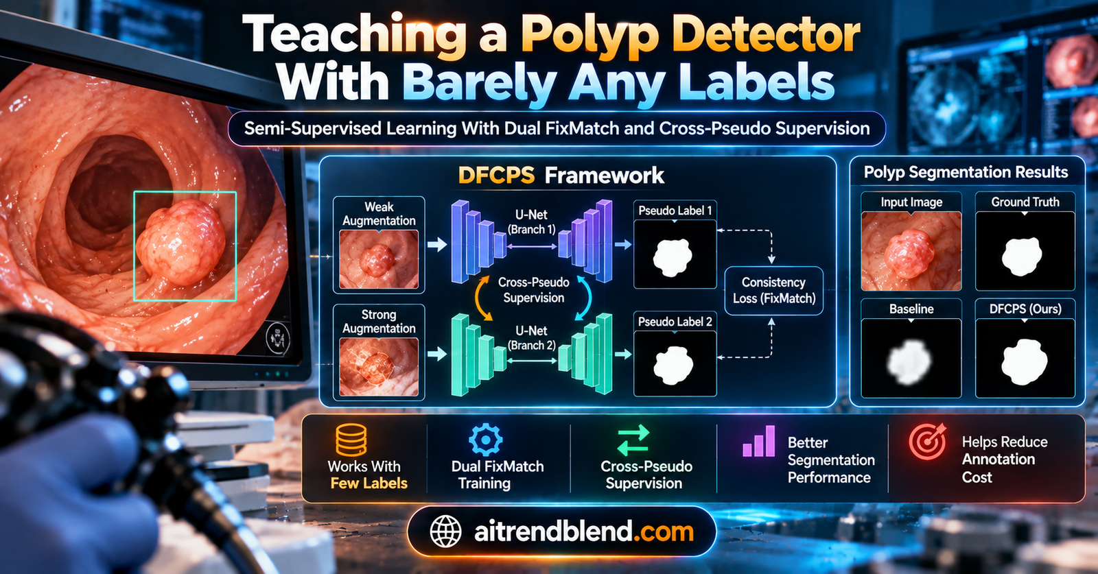
- DFCPS, short for Dual Fixmatch Cross Pseudo Supervision, is a semi-supervised segmentation model that combines strong and weak data augmentation with a mechanism the authors call cross-pseudo-supervision to squeeze more signal out of unlabeled images.
- Tested on the Kvasir-SEG polyp dataset with only one sixteenth of the images labeled, DFCPS reached a mean intersection over union of 72.39 percent, ahead of every baseline the authors compared it against at that same label fraction.
- The model runs four networks in two weight sharing pairs, each pair processing the same image at a different augmentation strength, and cross checks the pseudo labels each pair produces against the other pair.
- An ablation study found that pairing strong augmentation with weak augmentation beat every other combination tested, including no augmentation at all, which produced the weakest results across every label fraction.
- This is a research paper shared on arXiv, tested only on a single public endoscopy dataset, and it segments where a polyp is in a still image rather than diagnosing or classifying disease.
The real bottleneck in medical image AI is not compute, it is labels
Ask anyone who has tried to build a medical image segmentation model what the hardest part is, and the honest answer is rarely the neural network architecture. It is getting enough labeled data. A useful segmentation dataset needs pixel accurate outlines drawn by someone qualified to know what they are looking at, and for medical images that usually means a clinician’s time, which is expensive, limited, and not something a research team can simply buy more of at scale. Layer on top of that the practical realities the paper spells out directly, images that suffer from low light intensity, low signal to noise ratio, and poor contrast compared to ordinary photographs, plus organ deformation and individual patient variability that complicate the segmentation task itself, and plus the legal and ethical restrictions on sharing images that contain identifiable depictions of a patient’s body and condition. The end result, as the authors describe it, is that usable labeled datasets in this field tend to stay undersized no matter how much unlabeled imaging data exists in the world.
Semi-supervised learning exists precisely to work around this. The core idea is to make a small amount of labeled data go much further by also learning something useful from a much larger pool of unlabeled data, typically by having the model generate its own best guesses, called pseudo labels, for the unlabeled images and then training on those guesses as though they were real labels. The obvious risk is that a wrong guess reinforced as a confident target just teaches the model to be wrong. Most of the interesting engineering in this space is really about managing that risk, deciding which pseudo labels to trust and which to discard, and DFCPS is built directly on top of three prior ideas the authors credit explicitly.
Three ideas DFCPS borrows and recombines
FixMatch, originally proposed by researchers at Google Brain, is the simplest of the three and arguably the most influential. Its core trick is to compare a weakly augmented version of an unlabeled image against a strongly augmented version of the same image, using the weak version’s confident predictions as pseudo label targets for the strong version. The intuition is that a weakly augmented image, maybe just flipped or slightly rotated, is easier for the model to get right, so its predictions are more trustworthy, while training the model to match those predictions on a heavily distorted version of the same image forces it to learn features that are robust to real world variation rather than superficial shortcuts.
Cross Pseudo Supervision, abbreviated CPS and credited to Chen and colleagues, takes a different angle. It runs two separate networks with different random initializations, called perturbation networks, on the same input, and pushes their predictions to agree with each other through consistency learning, while also feeding pseudo labeled unlabeled data back into training as a self-training mechanism. Cross Probability Consistency, abbreviated CPC, is described in the paper as a streamlined adaptation of an earlier model called Guided Collaborative Training, retaining that model’s core structure while simplifying its constraints, and it also leans on consistency learning across unlabeled data using two constraints designed to be independent of the specific segmentation task.
DFCPS, whose full name is Dual Fixmatch Cross Pseudo Supervision, tries to take what works from all three. It keeps FixMatch’s strong versus weak augmentation contrast, keeps CPS’s idea of cross checking predictions between separate network branches, and wraps both around a more deliberate pseudo label generation, filtering, and refinement pipeline than either of its predecessors used on its own.
How the four networks talk to each other
The architecture is easiest to picture as two mirrored processing paths running on the same input image. In the first path, the image is strongly augmented and fed to one network, while a weakly augmented version of the same image is fed to a second network that shares its weights with the first. In the second path, the roles are reversed, weak augmentation goes to a third network and strong augmentation goes to a fourth, again sharing weights within that pair. That gives four networks total, organized into two weight sharing pairs, each pair seeing the same image at both augmentation strengths but through its own set of parameters.
Within a single pair, the weakly augmented branch’s prediction becomes the pseudo label target for the strongly augmented branch’s prediction, the same core mechanic as FixMatch. What makes this cross-pseudo-supervision rather than a simple repeat of FixMatch is the second layer of cross checking, where the pseudo labels generated by one pair’s weak branch are also used as targets to constrain the other pair’s predictions. In effect, each pair is being asked not only to make its own strong and weak predictions agree, but also to keep its pseudo labels consistent with what the other, independently weighted pair believes about the same image.
What is actually inside each network
Each of the four networks shares the same internal architecture, built on a ResNet-50 backbone. After the backbone extracts low level features, the output passes through an Atrous Spatial Pyramid Pooling module, borrowed from the DeepLabv2 architecture, which runs several parallel convolutional branches at different dilation rates alongside an image pooling branch, letting the model capture context at multiple spatial scales without the extra computational cost that simply using larger convolutional kernels would require. The outputs from all of these parallel branches are concatenated, passed through a sequence of convolution, pooling, batch normalization, and ReLU activation, then upsampled and merged back with the original low level features from the weakly augmented branch to form a richer combined representation. A pixel wise softmax over this combined representation produces the final segmentation prediction, in this case a binary decision between polyp and background for every pixel.
Batch normalization gets a specific mention in the paper as doing real work here, smoothing out what is called internal covariate shift, the tendency for the distribution of values flowing through a deep network to shift as earlier layers update during training, which in turn helps prevent vanishing or exploding gradients and generally stabilizes training.
The loss functions that hold it all together
Two loss functions drive the whole training process, a standard supervised loss for the labeled data and a cross-pseudo-supervision loss for the unlabeled data, and the way these interact is really the technical core of the paper.
The supervised loss averages pixel wise cross entropy loss \( l_{ce} \) across every labeled image in the labeled dataset \( D_l \), where \( S \) is the pixel area of the image, computed as height times width, and \( p_i, p_j \) are the confidence predictions from a pair of networks compared against the true ground truth labels \( y_i, y_j \).
The unlabeled data is where the more interesting mechanics happen, split across two separate terms that enforce two different kinds of consistency.
This term trains each pair’s strongly augmented prediction, \( P_{s1} \) or \( P_{s2} \), to match the pseudo label generated by that same pair’s weakly augmented branch, \( Y_1 \) or \( Y_2 \). This is the within pair mechanism, teaching the network to map a heavily distorted view of the image onto the same answer a gentler view already settled on.
This term instead swaps the pseudo labels across pairs, training the first pair’s weak prediction \( P_{w1} \) against the second pair’s pseudo label \( Y_2 \), and vice versa. This is the cross pair mechanism, the part that gives cross-pseudo-supervision its name, forcing two independently weighted branches of the network to agree with each other rather than just agreeing with themselves.
The total training objective sums the supervised loss with a weighted combination of both cross-pseudo-supervision terms, where \( \omega \) controls how strongly the unlabeled consistency signal factors into training relative to the labeled supervision.
One more detail matters a great deal in practice, though the paper describes it only briefly. Not every pseudo label gets used. The training pipeline applies a confidence threshold, and pseudo labels whose confidence sits too close to that threshold, meaning the model itself is not particularly sure about them, are discarded rather than fed into the loss calculation, while pseudo labels the model is confidently above threshold about are kept. This filtering step is exactly the kind of quality control that separates a semi-supervised method that actually works from one that quietly teaches itself to be confidently wrong.
The dataset, and what one sixteenth of it actually means
All of the experiments in this paper run on Kvasir-SEG, a segmented polyp dataset built from the broader Kvasir collection, described as the first multi category dataset designed for detecting and categorizing gastrointestinal diseases from endoscopic images, covering conditions such as polyps and ulcers with pixel level segmentation labels marking lesion boundaries. Kvasir-SEG specifically improves on the earlier Kvasir polyp category by replacing 13 of its original images with better ones. The researchers worked with a random selection of 1,000 intestinal polyp images from this dataset.
Following a data splitting protocol borrowed from the CPC baseline, the 1,000 images were divided by random selection into a labeled group and an unlabeled group, with the labeled group sized at one half, one quarter, one eighth, or one sixteenth of the full 1,000 images depending on which experimental condition was being tested, and everything not in the labeled group treated as unlabeled, deliberately simulating a label scarce clinical scenario. The one sixteenth condition, meaning roughly 62 labeled images standing in for the other 938, is the sharpest test of whether the semi-supervised machinery is actually earning its keep, since that is the setting where a purely supervised model would have the least to work with.
Training details, briefly
Training ran on a server with six NVIDIA GTX 2080Ti GPUs. The model was first pretrained on the PASCAL VOC 2012 dataset, a well known general purpose object segmentation benchmark unrelated to medical imaging, for 60 epochs at a base learning rate of 0.01, before the pretrained weights were transferred and fine tuned specifically on Kvasir-SEG for a further 100 epochs. Batch size was fixed at 12, with an adaptively adjusted learning rate ranging between a maximum of 1e-4 and a minimum of 1e-6.
How DFCPS performed against its competition
The authors compared DFCPS against the two methods it builds on directly, CPC and CPS, as well as two more recent methods described as state of the art, ELN and ACL-Net, all using the same ResNet-50 backbone for a fair comparison. Performance is reported as mean intersection over union, commonly abbreviated mIoU, a standard segmentation metric that measures how closely a predicted mask overlaps with the true mask, where a higher percentage means a closer match.
| Method | Half labeled | Quarter labeled | Eighth labeled | Sixteenth labeled |
|---|---|---|---|---|
| CPC | 77.91 | 76.10 | 73.01 | 67.36 |
| CPS | 78.47 | 76.74 | 75.66 | 70.50 |
| ELN | 75.23 | 73.14 | 71.19 | 71.12 |
| ACL-Net | 80.07 | 76.94 | 74.83 | 71.27 |
| DFCPS, the proposed model | 80.12 | 77.42 | 76.53 | 72.39 |
DFCPS leads at every single label fraction tested, though the size of its advantage varies quite a bit depending on how much labeled data is available. At the half labeled setting, DFCPS edges out ACL-Net by a slim 0.05 percentage points, hardly a decisive margin. The gap widens as labeled data becomes scarcer, reaching roughly a full percentage point ahead of ACL-Net and nearly two points ahead of CPS at the sixteenth labeled setting, which is exactly the pattern you would hope to see from a method specifically designed to make the most of scarce labels, even if the improvement at the easiest, most heavily labeled setting is modest enough that a reader should not treat every row of this table as equally convincing evidence of DFCPS’s advantage.
Training and inference time tell a more nuanced story than the accuracy table alone. DFCPS took 5.3 hours per epoch to train, slower than CPC’s 4.7 hours and CPS’s 5.1 hours, which the authors attribute to those two baselines skipping the feature consistency loss and its associated backpropagation steps that DFCPS’s cross-pseudo-supervision requires. Despite that heavier training cost, DFCPS came out fastest at inference time among every method compared, at 2.37 seconds per image against CPC’s 2.60, CPS’s 2.44, ELN’s 2.71, and ACL-Net’s 2.53. The authors frame that trade, a bit more training time in exchange for both better accuracy and faster inference once deployed, as a reasonable one, and the numbers support treating training cost and deployment cost as genuinely separate questions here.
What the ablation study actually shows
Perhaps the most informative table in the paper is not the main comparison but the ablation study, which isolates the effect of the augmentation pairing strategy itself by testing four combinations, the strong plus weak pairing DFCPS actually uses, a weak plus weak pairing, a strong plus strong pairing, and no augmentation at all using the original unmodified images.
| Augmentation pairing | Half labeled | Quarter labeled | Eighth labeled | Sixteenth labeled |
|---|---|---|---|---|
| Strong paired with weak, the DFCPS design | 80.12 | 77.42 | 76.53 | 72.39 |
| Weak paired with weak | 79.75 | 77.28 | 76.45 | 71.77 |
| Strong paired with strong | 79.63 | 77.04 | 76.28 | 71.23 |
| Original images, no augmentation | 78.47 | 76.74 | 75.66 | 70.50 |
The strong plus weak combination wins at every label fraction, confirming the core design choice, but the more interesting result sits in the middle two rows. Weak plus weak consistently outperforms strong plus strong, which is a genuinely useful, somewhat counterintuitive finding for anyone designing their own augmentation strategy, suggesting that pushing both branches through heavy distortion at once does more harm than good, likely because it makes both branches’ pseudo labels less reliable at the same time rather than giving the network a stable, trustworthy reference point to learn from. And unsurprisingly, skipping augmentation altogether produced the weakest results across the board, reinforcing that the augmentation contrast itself, not just the cross checking machinery layered on top of it, is doing real work.
The weak-weak enhancement combination outperformed the strong-strong enhancement combination. From the paper’s ablation experiment discussion, describing an asymmetry the authors found worth calling out explicitly
Clinical translation gap
It is worth stating plainly how far this sits from anything resembling a clinical tool. Every experiment in this paper runs on a single public dataset, Kvasir-SEG, drawn from one source collection of endoscopic images. The task itself is narrow and specific, pixel level segmentation of a polyp region that is already visible in a still image, which is a meaningfully different and much more constrained problem than detecting whether a polyp is present in a live video feed, distinguishing a polyp from other lesion types, staging a lesion’s severity, or making any kind of treatment recommendation. The paper’s own ethics statement confirms this is a retrospective study using previously collected, open access, de-identified data, not a study involving new patient interactions or clinical decision making of any kind.
Nothing in this paper trains, tests, or claims to support an actual diagnostic pipeline. A segmentation mask that closely overlaps a labeled polyp boundary on a benchmark dataset says something valuable about the algorithm’s technical capability, but it says nothing on its own about how that same model would behave on video captured by different endoscope hardware, in a different hospital system, on a patient population with different demographics, or under the time pressure and lighting variability of a live procedure. Moving from this kind of benchmark result toward any real clinical decision support tool would require substantially more validation, including testing on data from multiple institutions and multiple endoscope manufacturers, prospective rather than purely retrospective evaluation, and the full regulatory clearance process any software intended to inform patient care would need to go through.
Honest limitations
Several constraints deserve to be stated using only what the paper itself reports. The entire evaluation rests on 1,000 images from a single dataset, and while that dataset is a respected, purpose built resource for polyp segmentation research, a sample of this size from one source cannot speak to how the model generalizes to endoscopy images captured with different equipment, different lighting protocols, or patient populations with different demographic or clinical characteristics than whatever population Kvasir-SEG’s images were originally drawn from. The task is also strictly binary, polyp against background, so the paper offers no evidence about performance on multi class problems such as distinguishing polyp types or segmenting multiple simultaneous findings in one image.
The comparison table itself deserves a careful read rather than a glance at the bold winning number. DFCPS’s margin over the next best method, ACL-Net, is under a tenth of a percentage point at the most heavily labeled, easiest setting, which is a difference well within the kind of run to run variation common in deep learning experiments, and the paper does not report confidence intervals, standard deviations, or results averaged across multiple random seeds for any of its comparison tables, so it is not possible from the reported numbers alone to judge how much of the smaller gaps reflect a genuine, repeatable advantage versus noise from a single training run. The larger gap at the sparsest, one sixteenth labeled setting is more convincing simply because it is a bigger number, but the same caveat about run to run variance applies there as well.
Finally, this paper is presented as a preprint on arXiv. The text provided does not name a peer reviewed journal or conference venue, so readers should treat its claims with the appropriate caution generally extended to work that has not yet, or has not visibly, completed independent peer review, while recognizing that arXiv preprints in computer vision are a normal and common way for research to circulate before or alongside formal publication.
Where this points next
The paper does not spend much space speculating about future work, but the design itself suggests some natural directions. The confidence threshold used to filter unreliable pseudo labels is described only briefly, and how sensitive DFCPS’s results are to that threshold’s exact value is not explored in the reported experiments, which would be a natural next question for anyone trying to reproduce or extend this work. Testing across additional medical imaging datasets beyond a single endoscopy collection, and across imaging modalities beyond RGB endoscopy images, such as CT or MRI, would also be a reasonable way to establish whether the strong plus weak, cross pair supervision design generalizes as a general purpose semi-supervised strategy or whether its advantage is specific to the particular characteristics of polyp segmentation.
Conclusion
The contribution here is narrow and well scoped, which is exactly what makes it useful. DFCPS does not claim to solve medical image segmentation generally, or to replace a clinician’s judgment, or to diagnose anything. What it demonstrates, on one public benchmark, is that combining two already established semi-supervised ideas, FixMatch’s strong versus weak augmentation contrast and cross pseudo supervision’s dual network consistency checking, in a specific, deliberately engineered way produces a measurable improvement over either idea used alone, and a larger improvement still over both of the more recent baselines the authors compared against, particularly as labeled data becomes scarce.
The most transferable idea in this paper is arguably the ablation result rather than the headline architecture. Finding that weak plus weak augmentation beats strong plus strong, and that both beat no augmentation at all, is a concrete, actionable piece of guidance for anyone designing a pseudo labeling pipeline of their own, regardless of whether they use this exact four network, two loss term architecture. It suggests that the reliability of the pseudo label you are training against matters more than simply maximizing how much augmentation diversity you throw at the problem, a nuance easy to miss if you only look at the top line accuracy table.
The two cross-pseudo-supervision loss terms are the paper’s more durable technical idea. Separating within pair consistency, mapping a weak prediction onto a strong one, from cross pair consistency, forcing two independently weighted branches to agree, gives the training signal two genuinely different sources of error correction rather than one signal wearing two hats. That distinction is worth understanding even for readers who never touch this specific codebase, because the same logic, more than one independent source of consistency checking beats a single one, shows up across a lot of the semi-supervised and self-training literature.
What keeps this a research contribution rather than a deployment story is exactly what the paper does not claim. A single dataset, a single binary task, no reported variance across repeated runs, and no clinical validation of any kind. None of that diminishes what was actually shown, a real, reproducible improvement in a controlled benchmark setting, but it does mean the distance between this result and anything a patient or clinician would encounter directly remains substantial, and the paper itself, through its narrow scope and its own ethics statement describing a retrospective study on open access data, does not suggest otherwise.
For a field where the labeled data bottleneck is not going away anytime soon, methods like this one matter less for any single accuracy number and more for the accumulating evidence that careful pseudo label generation, filtering, and cross checking really can extract usable signal from unlabeled medical images. That is a genuinely useful direction of travel, even while the road from a 1,000 image polyp benchmark to a validated clinical tool remains long.
Reference implementation of the core training loop in PyTorch
The following is an original, simplified, runnable PyTorch implementation inspired by the dual branch architecture, the two cross-pseudo-supervision loss terms, and the confidence based pseudo label filtering described in the paper. It is a compact educational reconstruction of the core training mechanics, not the authors’ own code, built to illustrate the approach on dummy data with a working smoke test.
# dfcps_training_core.py
# Educational reimplementation of the DFCPS dual branch architecture,
# the supervised and cross-pseudo-supervision loss terms, and confidence
# based pseudo label filtering, inspired by "Semi-Supervised Medical
# Image Segmentation Method Based on Cross-Pseudo Labeling Leveraging
# Strong and Weak Data Augmentation Strategies", arXiv:2402.11273.

import torch
import torch.nn as nn
import torch.nn.functional as F

NUM_CLASSES = 2  # binary segmentation, polyp versus background
CONFIDENCE_THRESHOLD = 0.75


class SegmentationBranch(nn.Module):
    """A compact stand in for the ResNet-50 plus ASPP segmentation head
    described in Section 2.2. Two branches with shared weights form
    one of the paper's two weight sharing pairs."""
    def __init__(self):
        super().__init__()
        self.backbone = nn.Sequential(
            nn.Conv2d(3, 32, 3, padding=1), nn.BatchNorm2d(32), nn.ReLU(),
            nn.Conv2d(32, 64, 3, padding=1), nn.BatchNorm2d(64), nn.ReLU(),
        )
        # A small stand in for the ASPP module's multi-rate atrous branches.
        self.aspp = nn.ModuleList([
            nn.Conv2d(64, 32, 3, padding=rate, dilation=rate)
            for rate in (1, 12, 24, 36)
        ])
        self.head = nn.Conv2d(32 * 4, NUM_CLASSES, 1)

    def forward(self, x):
        features = self.backbone(x)
        multi_scale = [F.relu(branch(features)) for branch in self.aspp]
        fused = torch.cat(multi_scale, dim=1)
        logits = self.head(fused)
        return logits  # raw per pixel class scores, softmax applied by the caller


def weak_augment(x):
    """Placeholder for random rotation and horizontal translation as
    described in Section 2.2. Real training code would replace this
    with an actual augmentation pipeline."""
    return torch.flip(x, dims=[-1]) if torch.rand(1).item() > 0.5 else x


def strong_augment(x):
    """Placeholder for a heavier distortion than weak_augment. Real
    training code would use color jitter, cutout, or similar."""
    noise = torch.randn_like(x) * 0.15
    return torch.clamp(x + noise, 0.0, 1.0)


def filter_confident_pseudo_labels(probs, threshold=CONFIDENCE_THRESHOLD):
    """Implements the confidence threshold filtering described at the
    end of Section 2.3. Pixels whose top class probability does not
    clear the threshold are masked out of the pseudo label loss."""
    confidence, pseudo_label = probs.max(dim=1)
    reliable_mask = (confidence >= threshold).float()
    return pseudo_label, reliable_mask


def masked_cross_entropy(logits, pseudo_label, reliable_mask):
    """Pixel wise cross entropy, following the l_ce term used in every
    loss equation in the paper, restricted to confidently labeled
    pixels only."""
    per_pixel_loss = F.cross_entropy(logits, pseudo_label, reduction="none")
    if reliable_mask.sum() == 0:
        return torch.tensor(0.0, device=logits.device)
    return (per_pixel_loss * reliable_mask).sum() / reliable_mask.sum()


class DFCPSModel(nn.Module):
    def __init__(self):
        super().__init__()
        # Two weight sharing pairs, following Fig. 1 and Fig. 2 in the paper.
        self.pair_one = SegmentationBranch()
        self.pair_two = SegmentationBranch()

    def supervised_loss(self, x_labeled, y_labeled):
        """Implements Eq. 1, L_S, comparing both pairs' predictions on
        labeled data against the true ground truth labels."""
        logits_i = self.pair_one(x_labeled)
        logits_j = self.pair_two(x_labeled)
        loss_i = F.cross_entropy(logits_i, y_labeled)
        loss_j = F.cross_entropy(logits_j, y_labeled)
        return loss_i + loss_j

    def cross_pseudo_supervision_loss(self, x_unlabeled, omega=1.0):
        """Implements Eq. 2, Eq. 3, and Eq. 4, the within-pair and
        cross-pair consistency terms on unlabeled data."""
        x_strong_1, x_weak_1 = strong_augment(x_unlabeled), weak_augment(x_unlabeled)
        x_weak_2, x_strong_2 = weak_augment(x_unlabeled), strong_augment(x_unlabeled)

        logits_s1 = self.pair_one(x_strong_1)
        logits_w1 = self.pair_one(x_weak_1)
        logits_w2 = self.pair_two(x_weak_2)
        logits_s2 = self.pair_two(x_strong_2)

        probs_w1 = F.softmax(logits_w1, dim=1)
        probs_w2 = F.softmax(logits_w2, dim=1)
        y1, mask1 = filter_confident_pseudo_labels(probs_w1)
        y2, mask2 = filter_confident_pseudo_labels(probs_w2)

        # Eq. 2: within-pair, strong branch trained toward its own pair's pseudo label.
        l_cps_u = masked_cross_entropy(logits_s1, y1, mask1) + masked_cross_entropy(logits_s2, y2, mask2)

        # Eq. 3: cross-pair, weak branch of one pair trained toward the other pair's pseudo label.
        l_cps_l = masked_cross_entropy(logits_w1, y2, mask2) + masked_cross_entropy(logits_w2, y1, mask1)

        return omega * (l_cps_l + l_cps_u)

    def training_step(self, x_labeled, y_labeled, x_unlabeled, omega=1.0):
        """Implements Eq. 4, the total DFCPS training objective."""
        l_s = self.supervised_loss(x_labeled, y_labeled)
        l_cps = self.cross_pseudo_supervision_loss(x_unlabeled, omega=omega)
        total = l_s + l_cps
        return total, {"supervised_loss": float(l_s), "cross_pseudo_supervision_loss": float(l_cps)}


def smoke_test():
    """Runs one forward and backward pass on random dummy data to confirm
    every module is wired together correctly."""
    torch.manual_seed(0)
    model = DFCPSModel()
    optimizer = torch.optim.Adam(model.parameters(), lr=1e-4)

    batch, height, width = 2, 64, 64
    x_labeled = torch.rand(batch, 3, height, width)
    y_labeled = torch.randint(0, NUM_CLASSES, (batch, height, width))
    x_unlabeled = torch.rand(batch, 3, height, width)

    loss, logs = model.training_step(x_labeled, y_labeled, x_unlabeled, omega=0.5)
    optimizer.zero_grad()
    loss.backward()
    optimizer.step()

    print("Total loss", float(loss))
    print("Loss components", logs)
    print("Smoke test completed without errors")


if __name__ == "__main__":
    smoke_test()
Frequently asked questions
What does DFCPS actually do
DFCPS segments the pixel boundaries of polyps in endoscopic images, meaning it outputs a mask marking which pixels belong to a polyp and which belong to background tissue. It is designed to learn this task well even when only a small fraction of the training images have hand drawn ground truth masks available, by also learning from unlabeled images through a pseudo labeling process.
What is a pseudo label and why does the model filter them
A pseudo label is a prediction the model makes on an unlabeled image, which is then used as a stand in training target as though it were a real, human drawn label. Because the model can be wrong, especially early in training, DFCPS applies a confidence threshold and discards pseudo labels the model is not sufficiently confident about, only training on pseudo labels that clear that threshold.
Does DFCPS diagnose colon cancer or classify polyp type
No. The task tested in this paper is binary segmentation, distinguishing polyp pixels from background pixels in a still endoscopic image. The paper does not report any experiments on classifying polyp type, staging disease severity, or making any diagnostic or treatment related prediction.
How much labeled data does DFCPS need to work well
The paper tested DFCPS using as little as one sixteenth of a 1,000 image dataset as labeled data, roughly 62 images, with the rest treated as unlabeled. At that setting DFCPS reached a mean intersection over union of 72.39 percent, ahead of every baseline method tested at the same label fraction, though the paper does not test fractions smaller than one sixteenth.
What dataset was used to test the model
All experiments used Kvasir-SEG, a publicly available segmented polyp dataset built from the broader Kvasir collection of endoscopic gastrointestinal images. The researchers used a random selection of 1,000 images from this dataset, split into labeled and unlabeled groups at different ratios to simulate label scarce conditions.
Is this paper peer reviewed
The version of the paper reviewed for this article was shared as a preprint on arXiv. The text does not state a confirmed peer reviewed journal or conference venue, so this article treats it as a preprint rather than asserting formal peer review, consistent with how arXiv preprints in computer vision commonly circulate before or alongside formal publication.
Read the original research
This analysis is based on the preprint shared on arXiv in February 2024.
Pingback: Unlock 5.7% Higher Accuracy: How KD-FixMatch Crushes Noisy Labels in Semi-Supervised Learning (And Why FixMatch Falls Short) - aitrendblend.com