
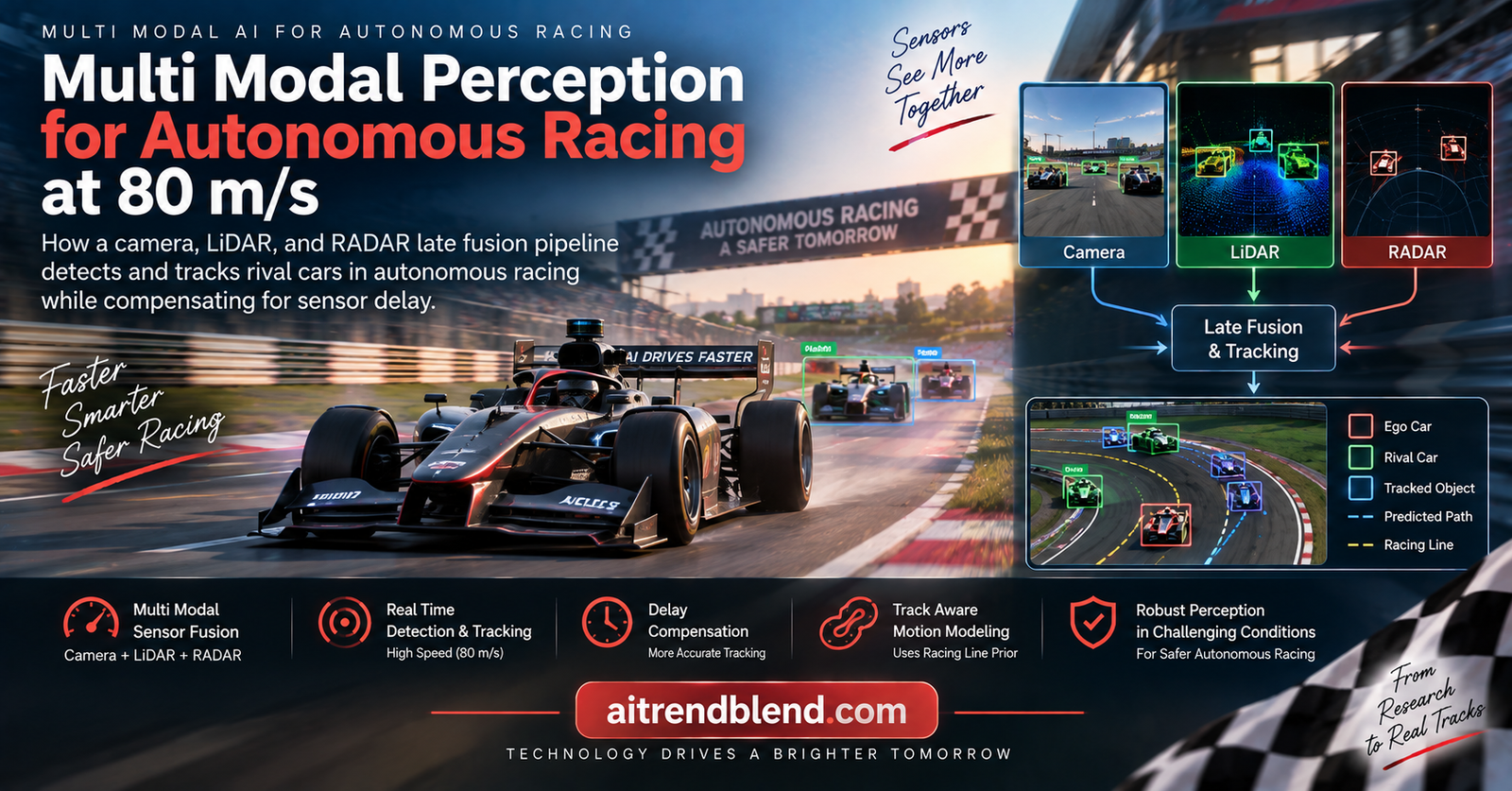
Two driverless race cars are closing on each other at a combined speed that would cross a football field in under a second. One has to decide whether the gap ahead is an overtaking chance or a crash waiting to happen, and it has to decide now, because a tenth of a second of hesitation is eight meters of uncertainty about where the other car actually is. A team from the University of Modena and Reggio Emilia, racing under the UNIMORE Racing banner, built the perception system that has to survive exactly this, and they ran it in real competition.
Key points
- At speeds near 80 meters per second, a 100 millisecond sensor delay translates to almost 8 meters of position error, so latency is a safety problem, not a performance detail.
- The system fuses cameras, LiDARs, and RADARs late, after each sensor has produced its own detections, so a single sensor failure degrades the system rather than blinding it.
- Each sensor covers the others’ weak spots, cameras for range, LiDAR for precise 3D depth, and RADAR for direct velocity from the Doppler effect.
- A tracker works in track relative coordinates and leans on a precomputed racing line, so its motion prediction already knows the car should slow into corners and accelerate out.
- The pipeline ran on a real car at the 2025 Abu Dhabi Autonomous Racing League event, and an ablation confirms each sensor contributes a distinct strength.
Why speed changes the whole problem
Autonomous perception is usually described in terms of accuracy. Did the system find the object, and did it draw the box in the right place. In racing, that framing is incomplete, because the clock is part of the problem. At the speeds these cars reach, close to 80 meters per second, the world moves faster than the sensors can report on it. A delay of 100 milliseconds, which is nothing in most vision systems, corresponds to nearly 8 meters of spatial error by the time the measurement is used. A detection that was perfectly accurate when it was captured is badly wrong by the time it reaches the planner.
This turns several ordinary engineering choices into critical ones. Sensors run asynchronously, each on its own clock, so their measurements never quite line up in time. Detection pipelines take milliseconds to run, and those milliseconds are meters. Relative velocities between cars are enormous, so any error in estimating an opponent’s speed compounds quickly into an error in predicting where it will be. The paper frames the whole effort around this reality, that in extreme speed environments, timing and delay matter as much as raw detection quality, and a system that ignores delay will make confident, dangerous mistakes.
The setting is real, not simulated. The pipeline was deployed by UNIMORE Racing at the 2025 Abu Dhabi Autonomous Racing League event on the Yas Marina Circuit, running on a Dallara EAV-24 race car. That grounding matters, because racing exposes edge cases, a stalled car appearing at high closing speed, an opponent hidden behind the car you are chasing, two cars running side by side at the limit, that also show up in ordinary autonomous driving but rarely get tested at this intensity.
Three sensors, three different strengths
The car carries a deliberately redundant sensor suite, three LiDARs, seven cameras, four RADARs, plus a dual antenna satellite navigation and inertial unit for localization. The design principle behind combining them is late fusion, which means each sensor first produces its own object detections independently, and only then are those detections merged. The alternative, early fusion, would blend raw sensor data before detection, but late fusion buys two things the authors care about. It is flexible, because you can change one sensor’s detector without redesigning the whole system, and it is robust, because if one sensor fails the others keep producing detections and tracking continues.
Each sensor earns its place by being good at something the others are not.
Cameras for reach and recognition
Camera detection uses YOLOv4, pretrained on the open road dataset BDD100k and then fine tuned on a custom set that mixes online videos of human driven open wheel race cars with roughly 600 manually labeled images from earlier test sessions. Seven cameras are processed as a batch, and the pipeline is optimized with the tkDNN framework and TensorRT to reach an average inference time of 4.5 milliseconds for all seven images on an RTX 6000 Ada GPU. Cameras see far, which matters when LiDAR range runs out, but a single camera cannot measure depth precisely, so its distance estimates degrade with range.
LiDAR for precise 3D geometry
LiDAR detection uses PointPillars, pretrained on the KITTI dataset and adapted with a custom set of nearly 25,000 manually labeled point clouds from previous race events. The three LiDAR scans are merged into a single point cloud, and the detector outputs 3D boxes with position, orientation, and size. A nice detail handles the timing problem at the source, since LiDAR points within a single scan are captured at slightly different instants, the detection timestamp is set to the average of all contributing points, giving the tracker a more precise time reference. LiDAR inference runs in 8.4 milliseconds on the same GPU. Its weakness is range, beyond its effective distance there simply are no points.
RADAR for direct velocity
RADAR does not use a neural network at all. It filters the raw point cloud by radar cross section, signal to noise ratio, and the existence probability the sensor assigns each point, which removes ghosts and reflections, then discards points outside the track using the car’s own localization. A simple clustering step groups the survivors by distance and velocity, keeping only clusters with enough points, and the whole thing runs in under 3 milliseconds per point cloud. RADAR’s gift is the Doppler effect, it measures an object’s radial velocity directly rather than inferring it from position changes over time, which is exactly the quantity that is hardest to estimate well at racing speeds.
How the detections get merged
Fusion happens pairwise, for every pair of detections from different sensors whose fields of view overlap. The first check is temporal, the two detections must be close enough in time, within a maximum gap, before they are even considered a candidate match. Then the merging depends on which sensors are involved.
Camera and LiDAR matching is the most involved. For a 2D box in a camera image, the system takes LiDAR points in the overlapping field of view, removes the ground plane by fitting a local plane to each point’s neighbors and filtering by the surface normal, drops points above a height threshold and points belonging to the car itself, and then projects the remaining points into the camera image using the calibrated transform, camera intrinsics, and lens distortion.
Only LiDAR points that land inside the 2D box are kept, a histogram of their ranges is built, and the most populated bin becomes the object’s distance. That distance turns the 2D camera box into a 3D world detection. Camera and RADAR matching works the same way minus the ground removal, and it adds the object’s radial velocity from the RADAR cluster. LiDAR and RADAR matching augments a 3D LiDAR box with the radial velocity of the RADAR points that fall inside it. The result of all this is a set of fused detections that each carry the best available estimate of position, size, and velocity.
Tracking that knows the track
The cleverest part of the system is the tracker, and its key idea is that a race car is not a free object moving through open space. It is constrained to a track whose geometry is known in advance. So rather than tracking opponents in raw Cartesian coordinates, the system tracks them in Frenet coordinates defined relative to a precomputed racing line, a reference path with an associated speed profile that says how fast a car should be going at each point.
Each tracked object is described by four numbers, its position along the racing line, its sideways displacement from that line, and its longitudinal and lateral velocities. An Extended Kalman Filter maintains this state. The orientation of the opponent is read off the racing line at the object’s position, a sensible choice because only the LiDAR detector directly measures orientation, so leaning on the track geometry keeps the estimate stable even if LiDAR drops out. This kind of state estimation over a maintained history is close in spirit to work on online tracking that reasons from memory rather than the current frame alone.
The motion model is where prior knowledge enters. Instead of assuming an opponent moves at constant velocity, the tracker uses a modified model whose predicted velocities drift toward reference values taken from the racing line’s speed profile.
The reference inputs come from the speed profile, so the model naturally captures deceleration into a corner and acceleration out of it, and the time constants control how fast the prediction relaxes toward those references. This embeds racing knowledge directly into the prediction step, which is more realistic than assuming an opponent will keep doing whatever it was just doing.
A race car is not a free object in open space. It is bound to a track whose shape and speed profile are known, and a tracker that assumes as much predicts far better than one that starts from nothing. Reading of the Frenet racing line tracker
Compensating for delay
The lifecycle of a tracked object is where delay compensation lives. Detections are associated to existing tracks using the Munkres assignment algorithm on Euclidean distance. When a detection arrives late, which at these speeds it always somewhat does, the system reverts the relevant track’s state back to the past instant the detection actually describes, inserts the correction there, and then replays the correction history forward to the current time. A new object is initialized with the detection’s position and the ego vehicle’s velocity, since two cars on the same track tend to move at similar speeds, with a high initial uncertainty, and it is only confirmed after a handful of consistent corrections to guard against spurious detections.
What the experiments show
Evaluation used real data from the 2025 event, with high quality localization shared between participating cars serving as ground truth. Errors are reported in track coordinates, split into longitudinal error along the direction of motion and lateral error across the track, which is more meaningful for racing than a single blended number. The ablation, run on a 315 second sequence of chasing another car at high speed, isolates what each sensor contributes.
| Configuration | Longitudinal RMSE | Lateral RMSE | Velocity RMSE | Max range |
|---|---|---|---|---|
| LiDAR and RADAR | 1.17 m | 0.41 m | 0.95 m/s | 73.05 m |
| Camera and RADAR | 1.72 m | 0.53 m | 1.13 m/s | 95.15 m |
| Camera and LiDAR | 1.54 m | 0.42 m | 1.43 m/s | 76.91 m |
| All three sensors | 1.40 m | 0.41 m | 0.77 m/s | 96.0 m |
The story reads cleanly across the rows. Dropping LiDAR, the camera and RADAR pairing, hurts both position errors, which confirms LiDAR’s role in precise depth where a monocular camera guesses. Dropping RADAR, the camera and LiDAR pairing, sends the velocity error up to 1.43 meters per second, which confirms RADAR’s Doppler measurement as the source of good velocity estimates. The LiDAR and RADAR pairing actually posts the lowest longitudinal error at 1.17 meters, but it gives up range. The full configuration has a slightly higher longitudinal error, 1.40 meters, precisely because it tracks objects out to 96 meters where only camera and RADAR reach and their estimates are looser, yet it wins the balance that matters, the lowest velocity error at 0.77 meters per second, the best lateral accuracy, and the longest tracking range and duration.
Three case studies fill in the behavior under the scenarios that actually threaten a race. In a high relative speed overtake, a stopped car is first seen at about 80 meters while the ego car approaches at nearly 60 meters per second, and the tracker confirms the new object 150 milliseconds after first detection, by which point it is 68.81 meters away, and its velocity has converged to near zero in time for the planner to react before the time to collision reaches one second. In a multi object case, an opponent hidden behind the car being chased suddenly appears at about 52 meters when the ego car pulls out to overtake, and its velocity converges within two iterations. In a side by side overtake at a minimum lateral gap of 1.75 meters, the system holds the track through the closest and most dangerous phase of a pass.
Honest limitations
The side by side case also exposes the system’s clearest weakness, and the authors lay it out plainly. The longitudinal estimate carries a bias that depends on where the opponent is relative to the ego car, reaching up to 0.84 meters. The cause is that camera detections have no semantic awareness of which part of the opponent they are seeing. When the opponent is ahead, the camera mostly sees its rear and underestimates how far forward it is, and when the opponent is behind, the camera sees its front and overestimates. Without knowing which end of the car is in view, the tracker cannot fully correct this, and the lateral error picks up a similar bias up to 0.61 meters when the cars are aligned.
The racing line prior, so helpful for prediction, also introduces its own error. Because the tracker assumes an opponent follows a stored racing line, when the opponent takes a wider line than expected the inferred heading can be off by as much as 9 degrees. The prior that makes normal prediction better makes atypical maneuvers harder to read. There is also an honest note on data, the training and validation datasets are relatively small, so the detectors would benefit from evaluation on larger benchmarks before strong generalization claims are made.
Finally, this is a report on a deployed system rather than a controlled study with many trials. The scenarios are representative and the ground truth is credible, but they are individual cases from a live event, so the numbers describe what happened on that track with those cars rather than a statistical distribution over many runs. That is the right way to read a racing deployment paper, as evidence that the system works under real pressure, not as a precise benchmark of how it would rank against alternatives.
Why the approach travels
Two ideas here reach well past motorsport. The first is that redundancy through late fusion is a robustness strategy, not just an accuracy one. By keeping each sensor’s detection independent and merging afterward, the system stays alive when a sensor drops, and it can be modified one piece at a time. Any safety critical perception system, from a delivery robot to a driver assistance stack, benefits from that separation, and it is a discipline worth adopting even when a fancier early fusion scheme might squeeze out a little more accuracy.
The second is that domain priors belong in the estimator. The tracker is good not because its filter is exotic but because it knows the car is on a track and uses the racing line to shape its predictions. Encoding what you already know about the world, the geometry, the constraints, the expected behavior, into the estimator rather than hoping the model learns it from data is a pattern that shows up across robotics, including planning work like motion planning for dense robot swarms. The same instinct, that latency is a first class concern, applies to any system where the world changes faster than the pipeline can report on it.
Conclusion
This paper is a systems result grounded in a hard reality. Autonomous racing compresses every perception problem into a few milliseconds and a few meters, and it punishes any design that treats timing as an afterthought. The team’s answer is a late fusion pipeline that combines cameras, LiDARs, and RADARs, paired with a tracker that compensates for delay and reasons in the coordinate frame of the track itself. None of the individual pieces is novel in isolation, but assembling them into a delay aware, racing aware whole and running it in real competition is the contribution.
The conceptual through line is that prior knowledge is leverage. The system knows the track layout, so it tracks in racing line coordinates and predicts with a speed profile. It knows that sensors are delayed, so it reverts and replays state to place each measurement at the moment it truly describes. It knows that no single sensor is complete, so it fuses three that cover each other’s blind spots. Each of these is a way of building what is known about the world into the pipeline rather than hoping to recover it from raw data at 80 meters per second.
The evidence is honest about what it is. The ablation cleanly attributes a distinct strength to each sensor, LiDAR for depth, RADAR for velocity, cameras for range, and shows the full combination striking the best overall balance. The case studies show the system handling the scenarios that matter, high closing speeds, occluded opponents, and side by side passes, at meter level and sub meter level accuracy. These are real deployment results, not controlled benchmarks, and the paper reads them that way.
The limitations point somewhere specific and useful. The dominant remaining error comes from the camera not knowing which part of the opponent it sees, and the racing line prior that helps normal prediction hurts when an opponent behaves atypically. Both are addressable, the first with semantic vehicle geometry, the second with more flexible trajectory priors, and the authors name both as future work.
For anyone building perception for fast moving autonomous systems, the lessons are concrete. Treat latency as a safety variable and design compensation for it from the start. Fuse complementary sensors late so a failure degrades rather than blinds the system. And put what you know about the world into the estimator, because a tracker that understands the track will always outpredict one that does not. Racing is an extreme test bed, which is exactly why a system that survives it has something to teach the calmer world of everyday autonomy.
Reference implementation in Python
The code below is a compact, runnable sketch of the tracking ideas, a Frenet coordinate state with the modified constant velocity process model, an Extended Kalman Filter predict and update step, racing line matching by cumulative distance, and delay compensation by reverting and replaying state, with a smoke test on dummy data. It captures the mechanics for study rather than reproducing the authors’ full fusion and detection stack.
# racing_tracker.py
# Study reference for the autonomous racing tracker ideas, a Frenet state EKF
# with a racing line speed prior plus delay compensation. Not the authors' full
# pipeline. Runs a smoke test on dummy data at the end.

import numpy as np


class RacingLine:
    """A reference path with a speed profile, indexed by arc length s."""
    def __init__(self, s_grid, speed_profile, xy):
        self.s = np.asarray(s_grid)
        self.speed = np.asarray(speed_profile)   # target longitudinal speed at each s
        self.xy = np.asarray(xy)                  # centerline points for matching

    def target_speed(self, s):
        return float(np.interp(s, self.s, self.speed))


class FrenetEKF:
    """EKF in Frenet coords, state = [s, d, v_s, v_d].
    Velocities relax toward racing line references, matching the paper's model."""
    def __init__(self, line, tau_vs=0.8, tau_vd=0.5):
        self.line = line
        self.tau_vs, self.tau_vd = tau_vs, tau_vd
        self.x = np.zeros(4)
        self.P = np.eye(4) * 10.0          # high initial uncertainty
        self.Q = np.diag([0.05, 0.05, 0.5, 0.5])
        self.R = np.diag([0.3, 0.3, 0.4])   # measure s, d, v_s

    def predict(self, dt):
        s, d, vs, vd = self.x
        u_vs = self.line.target_speed(s)         # reference from speed profile
        u_vd = 0.0                              # reference lateral velocity is zero
        # modified constant velocity update, eqs 1 to 4
        s = s + vs * dt
        d = d + vd * dt
        vs = vs + (u_vs - vs) / self.tau_vs * dt
        vd = vd + (u_vd - vd) / self.tau_vd * dt
        self.x = np.array([s, d, vs, vd])
        F = np.array([
            [1, 0, dt, 0],
            [0, 1, 0, dt],
            [0, 0, 1 - dt / self.tau_vs, 0],
            [0, 0, 0, 1 - dt / self.tau_vd]])
        self.P = F @ self.P @ F.T + self.Q

    def update(self, z):
        # measurement of s, d, v_s from fused detection
        H = np.array([[1, 0, 0, 0], [0, 1, 0, 0], [0, 0, 1, 0]])
        y = z - H @ self.x
        S = H @ self.P @ H.T + self.R
        K = self.P @ H.T @ np.linalg.inv(S)
        self.x = self.x + K @ y
        self.P = (np.eye(4) - K @ H) @ self.P


def match_racing_line(lines, recent_xy):
    """Pick the racing line minimizing cumulative distance to recent states."""
    best, best_cost = 0, float("inf")
    for i, line in enumerate(lines):
        cost = 0.0
        for p in recent_xy:
            d = np.linalg.norm(line.xy - p, axis=1).min()
            cost += d
        if cost < best_cost:
            best, best_cost = i, cost
    return best


def delay_compensated_update(ekf, history, z, t_meas, t_now, dt):
    """Revert to the measurement instant, correct, then replay to now."""
    steps_back = max(0, int(round((t_now - t_meas) / dt)))
    if steps_back < len(history):
        ekf.x, ekf.P = history[-1 - steps_back]   # revert to past state
    ekf.update(z)                                # apply the late measurement there
    for _ in range(steps_back):                    # replay forward to the present
        ekf.predict(dt)
    return ekf.x


def smoke_test():
    s_grid = np.linspace(0, 200, 201)
    speed = 60 + 10 * np.sin(s_grid / 30)         # faster on straights, slower in corners
    xy = np.stack([s_grid, np.zeros_like(s_grid)], axis=1)
    line = RacingLine(s_grid, speed, xy)
    ekf = FrenetEKF(line)
    ekf.x = np.array([10.0, 0.0, 55.0, 0.0])
    dt, history = 0.02, []
    for _ in range(10):
        ekf.predict(dt)
        history.append((ekf.x.copy(), ekf.P.copy()))
    print(f"predicted state s d vs vd {np.round(ekf.x, 2)}")
    z = np.array([ekf.x[0] - 1.0, 0.2, 58.0])       # a slightly delayed measurement
    x_now = delay_compensated_update(ekf, history, z, t_meas=0.10, t_now=0.20, dt=dt)
    print(f"after delay compensated update {np.round(x_now, 2)}")
    idx = match_racing_line([line], [np.array([50.0, 0.1])])
    print(f"matched racing line index {idx}")


if __name__ == "__main__":
    smoke_test()
Running the smoke test predicts a tracked opponent forward along a racing line whose speed profile pulls its velocity toward the corner and straight targets, applies a delayed measurement by reverting to the correct past instant and replaying to the present, and matches a track to a short history of positions. The delay compensation step is the one to watch, since reverting and replaying is what keeps a late measurement from being applied at the wrong place.
Frequently asked questions
Why is perception so hard in autonomous racing?
The cars move at close to 80 meters per second, so a 100 millisecond delay corresponds to nearly 8 meters of position error. Sensors run asynchronously and relative velocities are huge, which means timing and delay matter as much as raw detection accuracy.
What is late fusion and why use it here?
Late fusion means each sensor produces its own object detections first and the detections are merged afterward. It is flexible, because a single sensor’s detector can be changed without redesigning the system, and robust, because if one sensor fails the others keep the tracking alive.
What does each sensor contribute?
Cameras provide long range detection and recognition but weak depth, LiDAR provides precise 3D position and orientation within its range, and RADAR measures radial velocity directly through the Doppler effect. The ablation shows removing any one degrades a specific part of the estimate.
How does the tracker use knowledge of the track?
It tracks opponents in coordinates relative to a precomputed racing line and uses that line’s speed profile as the reference for its motion model, so its predictions already expect deceleration into corners and acceleration out of them rather than assuming constant velocity.
How does it handle sensor delay?
When a detection arrives late, the tracker reverts the affected object’s state to the past instant the detection describes, applies the correction there, and replays the correction history forward to the current time, so a delayed measurement is never applied at the wrong position.
What are the main limitations?
Camera detections do not know which part of the opponent they see, which biases the longitudinal estimate by up to about 0.84 meters, and the racing line prior can misjudge heading by up to 9 degrees when an opponent takes an atypical line. The training datasets are also relatively small.
Read the full paper for the complete pipeline and all three racing scenarios.
Read the paper on arXiv