
Key points
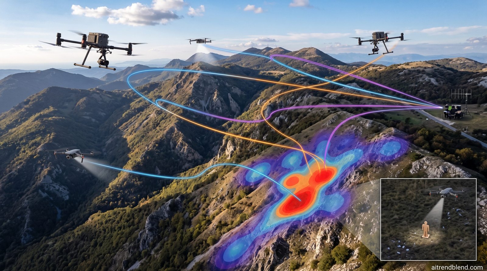
- The framework couples a probabilistic model of where a missing person might be with a two part control system, ergodic HEDAC control for horizontal search patterns and model predictive control for altitude and speed.
- Detection performance is tied to a real machine learning model’s recall curve rather than an assumed camera range, so the sensing math reflects what a YOLO based detector can actually see at a given altitude.
- Three simulated scenarios reached 98 percent, 96 percent, and 77 percent survey completion within their time budgets, and the method beat a lawnmower search pattern and two competing ergodic control variants in every case.
- A real field test on Mount Učka with two UAV types and 100 physical targets showed the predicted completion metric tracked the actual detection rate closely enough to be useful for a search coordinator on the ground.
- The detection curve used for human targets is borrowed and scaled from an animal detection study, and the field validation ran its detector at an unusually permissive confidence threshold, two choices worth understanding before anyone adapts this for an operational deployment.
Search and rescue missions live or die on speed. Every hour spent searching the wrong hillside is an hour a missing hiker does not have, and remote terrain, whether that is wilderness, a collapsed urban block, or open water, tends to punish slow or inefficient coverage patterns. Autonomous UAVs have been pitched as a fix for this for years, since a drone can cover ground a foot patrol cannot reach and does it without tiring. The catch has always been that flying well over flat, empty terrain is a solved problem, while flying well over a mountain, where altitude above sea level and altitude above the ground diverge constantly, is not.
Luka Lanča, Karlo Jakac, and Stefan Ivić, all with the Faculty of Engineering at the University of Rijeka, built a system that treats this as two coupled problems rather than one. Where should the aircraft go across the map, and how high above the terrain directly beneath it should it fly at that moment. Their answer links a heat equation based coverage algorithm to a receding horizon optimizer, backed by a probabilistic model that folds in how a real camera and a real detection model perform as altitude changes.
The core problem, searching a shape you cannot see
The starting assumption is that nobody knows exactly where the target is. What the searchers do have is a probability distribution over the search area, essentially a heat map of where a missing person is more or less likely to be, built from whatever tips, terrain, and prior information the search team has. A naive strategy just chases the brightest spot on that map. That works if the prior is accurate, and fails badly if it is not, since a greedy search can spend the whole mission circling one hillside while the person is actually two ridges over.
Ergodic search solves this differently. Instead of chasing the peak, the aircraft’s time spent in each region should match that region’s probability mass over the long run. High probability zones get visited more often, low probability zones still get swept, just less frequently. The formal definition, credited to the ergodic theorem, says a trajectory is ergodic with respect to a distribution if the time average of any test function along the path converges to the spatial average of that function weighted by the distribution. In plain terms, fly so that where you spend your time and where the target probably is line up asymptotically.
HEDAC, treating uncertainty like a temperature field
The specific ergodic method used here is called heat equation driven area coverage, HEDAC for short, first introduced by Ivić and coauthors and refined across several follow up papers, including applications to crop spraying, maze exploration, and even algorithmic portrait drawing. The trick is an analogy. Treat the undetected target probability as a heat source. Solve a steady state heat equation over the domain to get a potential field. The gradient of that potential field points toward where heat, meaning uncertainty, is currently concentrated. As the aircraft searches an area, it lowers the local heat source there, the potential field reshapes itself, and the gradient naturally redirects the aircraft elsewhere.
The governing equation is a Poisson type relation between the potential u and the undetected probability field m, with a smoothing parameter that controls whether the search behaves locally or globally, and a stability parameter with a weaker practical effect.
with a zero flux boundary condition so the field does not leak heat out of the search domain. The heading command for each aircraft comes from the normalized gradient of this field, adjusted by a yaw rate that respects the aircraft’s turning limits. It is an elegant piece of engineering because the same mechanism that tracks where the search has already been also handles the physical geometry of the domain, obstacles included, without a separate path planning layer bolted on.
Why altitude needed its own controller
Flat terrain lets a drone hold a constant height above sea level and call it done. Hilly terrain breaks that assumption immediately. The paper draws a careful distinction between height, which is relative to sea level, and altitude, which is relative to the ground directly underneath the aircraft. A UAV holding constant height over a ridge will end up flying dangerously close to the ground on the way up and uselessly far from it on the way down, which hurts both safety and detection quality at the same time.
The authors handle this with model predictive control layered on top of the ergodic heading command. Every control cycle, the system predicts a short horizontal path using the current potential field gradient, samples the terrain elevation along that predicted path, and then searches for a combination of velocity intensity and climb angle that keeps the aircraft as close as possible to a goal altitude above the ground while also flying as fast as safely possible.
The optimization balances two objectives without weighting one over the other. The velocity objective rewards using more of the available speed.
and the altitude objective penalizes drifting away from the goal altitude above whatever terrain is coming up.
Both are normalized so they carry comparable weight, then simply added. A separate hard constraint enforces the minimum safe altitude above ground, along with velocity and acceleration bounds that keep the trial trajectory physically achievable for the specific aircraft. The optimizer solves this with a mesh adaptive direct search method through the Indago Python package rather than gradient descent, since the objective involves discrete decisions about feasibility that do not play nicely with a smooth solver, and it caps itself at 30 iterations with early stopping so the whole loop finishes well inside the control time step.
Keeping multiple aircraft from colliding
With more than one UAV converging on the same probability hotspot, collision avoidance becomes unavoidable. The method checks each aircraft against bounding circles that contain every possible position it could reach given its range of feasible horizontal speeds, since the actual speed at the next step is not yet fixed. Only when a bounding circle check flags a potential conflict does the system spend the extra computation adjusting the yaw rate within its allowed range to steer clear, then verifies that an escape maneuver, a tight circular arc combined with maximum climb and minimum speed, remains available at every future instant. If the optimized flight parameters would leave no viable escape route, the aircraft is forced into the escape maneuver immediately rather than waiting for a near miss.
Turning a detection model’s recall curve into a sensing function
This is the part of the paper that separates it from a purely theoretical control exercise. The detection probability at any point is not assumed, it is derived from the recall of an actual computer vision model as a function of altitude. Recall is the fraction of real targets a detector actually finds, and the authors treat it as the bridge between control theory and what a camera equipped drone can genuinely accomplish.
The math converts a time varying detection rate into a probability of detection using an exponential relationship,
then defines a scene duration, essentially how long any given ground point stays inside the camera’s field of view as the aircraft flies over it, based on the goal altitude and the average cruising speed.
With that duration fixed, a known recall value at a given altitude can be inverted algebraically to recover the underlying sensing rate function that the ergodic and coverage math actually needs.
This is a genuinely useful engineering pattern for anyone building a similar system, since it means the control algorithm does not need to know anything about neural networks. It just needs a recall curve, sampled at a handful of altitudes, and it can back out the physics of how fast uncertainty gets resolved at each point in space.
Where the recall numbers actually came from
Here is where the abstract undersells what the paper is doing. For the simulated test cases, the authors did not train a human detection model from scratch. They pulled recall values from a published YOLOv4 study on large mammal detection from UAV imagery, then reduced those values by 30 percent as a rough correction for the added difficulty of detecting humans instead of large animals against varied backgrounds. They also introduced a hard cutoff, an altitude above which detection is assumed impossible outright, calculated from the pixel footprint a person would occupy in a 4K frame, working out to around 222 meters for their baseline camera configuration.
That is a defensible engineering shortcut for a simulation study, since building a bespoke human detection dataset just to validate a control algorithm would be a project of its own. But it does mean that the survey accomplishment numbers reported for the three simulated scenarios rest on a detection curve that was never actually measured for human targets in those specific conditions. Anyone treating the 98, 96, or 77 percent figures as a literal prediction of real world detection performance should read them as coverage of the sensing budget the system assumed, not as a validated human detection rate.
The field experiment is what actually tests the claim, because that is where the detector was trained on the real targets it needed to find instead of borrowed from a different species. Editorial observation on the paper’s methodology
What the simulations actually showed
Three test scenarios probed different aspects of the system. A synthetic domain nicknamed plastic world, deliberately built with exaggerated peaks and depressions to stress test the altitude controller, used three multirotor UAVs and reached 98 percent survey accomplishment inside 30 minutes. A survey of the real terrain around Mount Vesuvius near Naples used five multirotor UAVs split across two altitude and zoom configurations and reached 96 percent within 60 minutes, including a variant where the volcanic crater itself was declared a no fly zone to test constraint handling. A 7.5 square kilometer stretch of star dunes in Algeria, surveyed with just two fixed wing UAVs at a much higher goal altitude to cover the larger area, reached 77 percent in the same 60 minute window.
That gap between 96 to 98 percent on the two multirotor cases and 77 percent on the dune case is worth sitting with. It is not a failure of the control algorithm, it is arithmetic. Two fixed wing aircraft covering 7.5 square kilometers simply have less sensing budget per unit area than five multirotors working a smaller volcanic slope. The paper is upfront that deploying more aircraft would be the single biggest lever for closing that gap, but it does not simulate that scaling claim, it only asserts that HEDAC’s known scalability from prior work should support it.
| Scenario | UAV configuration | Search window | Survey accomplishment |
|---|---|---|---|
| Plastic world, synthetic terrain | 3 multirotor UAVs | 30 minutes | 98 percent |
| Mount Vesuvius | 5 multirotor UAVs, mixed altitude and zoom | 60 minutes | 96 percent |
| Star dunes, Algeria | 2 fixed wing UAVs | 60 minutes | 77 percent |
Against competing methods the picture is consistent. A HEDAC search run at a single fixed altitude, without the MPC layer, stalled completely on the two terrain heavy scenarios because the fixed height calculation, set to clear the tallest peak in the domain plus a safety margin, put the aircraft far too high over the rest of the terrain to detect anything reliably. A lawnmower style sweep pattern combined with the same MPC altitude controller was allowed relaxed acceleration limits and permitted collisions between aircraft just to make its coverage comparable, and it still underperformed. Two spectral ergodic control variants from earlier literature, SMC and a modified version called mSMC originally built for the MH370 search effort, came closer, with mSMC landing nearly on par with the proposed method but consistently a step behind.
The mountain test, and what it actually validated
The real proof came from two missions flown over Mount Učka in Croatia, using a DJI Matrice 210v2 and a DJI Mavic 2 Enterprise Dual, searching for 100 physical cardboard targets scattered across three concentric probability zones. This time the detection model was not borrowed. The team trained a YOLOv8 detector specifically on 1166 aerial images of the actual targets, totaling 27,600 labeled object instances, and validated it on a held out set of 674 images with 6,535 instances.
The validated detector reached a mean average precision of 0.68, a precision of 0.82, and a recall of 0.58, evaluated at a confidence threshold of 0.001. That last number is worth pausing on. A confidence threshold of 0.001 is extremely permissive, close to accepting almost any detection the model proposes rather than filtering for high confidence hits, which is common practice when a researcher wants to trace out the full precision recall curve but is not necessarily representative of the threshold an operator would actually fly with in the field. The recall figures that feed the sensing function in this experiment were therefore measured under conditions more forgiving than a typical deployment configuration would use, and a search team adopting a stricter operational threshold to reduce false alarms should expect a lower effective recall than the one baked into this validation.
What the mountain test genuinely confirmed is the relationship between the algorithm’s internal survey accomplishment metric and the actual measured target detection rate across the mission. The two tracked each other closely across both flights, which is the more important result here than any single completion percentage, because it means a search coordinator watching the survey accomplishment number tick upward on a screen has a reasonably trustworthy proxy for how many real targets are actually being found, not just how much ground has been nominally covered.
A quieter but telling detail
Despite the algorithm computing each control step in well under a second, the field trials ran with a control interval of three seconds. The bottleneck was not the math, it was the practical pipeline of image focusing, image capture, and reporting the capture back to the control loop. That is a useful reminder that a real time capable algorithm on paper still has to survive contact with actual camera hardware and radio links, and anyone planning to replicate this system on a comparable aircraft should budget for that same kind of latency rather than assuming the sub second computation time translates directly into a sub second field control loop.
Where the method runs into trouble
The authors are candid about two structural limitations. First, poorly matched parameters, specifically a camera field of view narrower than twice the minimum turning radius combined with a minimum altitude constraint, can trap an aircraft in an endless circular holding pattern around a point of interest instead of actually completing the search. Second, and more fundamentally, the whole approach explores a two dimensional surface, the terrain, rather than true three dimensional space. It cannot see under a forest canopy, and it becomes unreliable on very steeply sloped ground because the clearance guarantee is calculated once during initialization from the maximum terrain incline in the domain, rather than checked continuously against the nearest terrain point during flight, a deliberate tradeoff made to keep the real time computation manageable.
The fix the authors propose for both of these, tighter parameter tuning and onboard proximity sensors for terrain that exceeds the supported incline, is reasonable but was not tested as part of this paper. It is a roadmap, not a demonstrated fix.
What this means if you are building something similar
For a team assembling a comparable search system, three practical lessons stand out beyond the headline architecture. Deriving the sensing function algebraically from a measured recall curve, as this paper does, is a clean way to keep the control math decoupled from whatever detection model happens to be running onboard, and it means the detector can be swapped or retrained without touching the ergodic or MPC layers. Second, the gap between the simulated scenarios, built on a borrowed and scaled animal detection curve, and the field validated mission, built on a purpose trained detector, is a reminder to treat simulation accomplishment numbers as an upper bound on what a real detector under real conditions is likely to achieve. Third, budget hardware latency into the control loop from the start, since the field experiments here needed a control interval three times longer than the algorithm’s actual computation time purely to accommodate the camera and reporting pipeline.
Limitations worth keeping in view
Beyond the terrain incline and turning radius issues the authors describe directly, a few things are worth flagging for anyone evaluating this work critically. The correlation between predicted survey accomplishment and actual detection rate during the Mount Učka experiment is described qualitatively as notable, without a reported correlation coefficient or confidence interval, so the strength of that validation cannot be independently checked from the paper’s numbers alone. The comparative simulations against lawnmower search, SMC, and mSMC each appear to be single runs rather than repeated trials, leaving no measure of variance behind the reported performance gaps. And the human detection curve underlying the three main simulated scenarios is adapted from an animal detection study rather than measured directly, a compromise the authors state plainly but one that limits how literally the simulated survey accomplishment percentages should be read as human detection guarantees.
The bigger picture
Search and rescue robotics has spent years chasing better path planning algorithms in isolation from the sensing hardware that actually has to find the person. What makes this paper worth attention is the refusal to treat those as separate problems. The control law literally does not know what a good search pattern looks like until it has been told, mathematically, how a specific camera and a specific detection model perform at each altitude. That coupling is the paper’s real contribution, more than the specific choice of HEDAC or MPC, and it is a template that should transfer cleanly to other sensing modalities, thermal cameras for night searches, or multispectral sensors for locating debris, as long as someone can supply a comparable recall curve.
The conceptual shift, treating detection performance as a first class input to the control law rather than an afterthought bolted onto a generic coverage algorithm, is the part likely to outlast the specific equations in this paper. Whether HEDAC remains the ergodic method of choice or gets swapped for something else in five years, the idea that a search controller should be built around a measured sensing function rather than an assumed one is durable. The honest gaps, a borrowed detection curve for the simulations and a permissive confidence threshold in the field validation, do not undercut that contribution so much as mark where the next round of work needs to focus, closing the distance between the algorithm’s mathematical guarantees and what a camera bolted to a drone can actually promise in the field.
Read alongside prior HEDAC papers on crop spraying and structural inspection, this work also signals the algorithm’s maturity path, from abstract coverage demonstrations toward mission specific validation with real hardware and real detection pipelines. That is the harder, less glamorous half of robotics research, and it is where this paper earns its place. The full simulation code, terrain meshes, flight logs, and the trained detection model are published on the Open Science Framework, which means the recall curves, the borrowed animal detection scaling, and the confidence threshold choices described here can all be inspected directly rather than taken on faith. The link sits in the citation section below.
Frequently asked questions
What does ergodic search mean in this context
It means flying so that the amount of time spent in each part of the search area matches how likely a target is believed to be there, rather than only chasing the single most likely spot on the map.
What is HEDAC
Heat equation driven area coverage. It models the undetected target probability as a heat source and solves a steady state heat equation to produce a potential field whose gradient steers the search aircraft toward unresolved uncertainty.
Why does the system need model predictive control in addition to ergodic search
Ergodic search decides where to fly across the map. Model predictive control decides how high and how fast to fly at each moment so the aircraft stays close to its goal altitude above uneven ground while respecting velocity and acceleration limits.
How accurate was the method in real world testing
Across two missions on Mount Učka, the algorithm’s predicted survey accomplishment metric tracked the actual measured target detection rate closely, which the authors treat as validation that the metric is a reliable stand in for real detection progress during a live mission.
Can this work for detecting objects other than people
The framework itself is detector agnostic since it only needs a recall curve as a function of altitude. Swapping in a different trained detector, for debris, vehicles, or other targets, should not require changing the ergodic or MPC control layers.
What are the biggest limitations of this approach
It explores the terrain surface rather than true three dimensional space, so it cannot search beneath forest canopy and struggles on very steep slopes, and its clearance guarantee is calculated once from the domain’s maximum incline rather than checked continuously, which trades some safety margin for real time performance.
Read the full paper and access the terrain meshes, flight logs, and trained detection model.
Read The Paper Open Data RepositoryFull PyTorch implementation
The paper’s contribution is a control system rather than a trained classifier, so a faithful reproduction means implementing the sensing function, the coverage and undetected probability update, the HEDAC potential field solve, and the MPC altitude and velocity optimization. The code below expresses the HEDAC potential field as an iterative relaxation solve and the MPC step as a gradient based optimization using PyTorch autograd, standing in for the finite element solver and the GPS MADS optimizer the original authors used. Both substitutions are noted inline. A runnable smoke test at the bottom exercises the full pipeline on a synthetic terrain and confirms survey accomplishment rises monotonically, the MPC respects the minimum altitude constraint, and the sensing rate correctly declines with altitude.
"""
Reproduction of the core probabilistic search and control model from
"Probabilistic Modeling and Control for Multi UAV Search Over Uneven Terrain"
Lanca, Jakac and Ivic, IEEE Transactions on Robotics, 2026.

This is not a conventional trained neural classifier. The paper's contribution is a
probabilistic sensing model coupled with two control laws, ergodic HEDAC control
for heading and MPC for altitude and velocity. Both control laws are naturally
expressed as optimization problems, so this implementation uses PyTorch tensors
and autograd to solve them, which mirrors the spirit of the paper even though the
original authors used a finite element PDE solver and the Indago GPS MADS optimizer
rather than gradient descent. That substitution is called out inline wherever it
happens.
"""

import math
import torch
import torch.nn.functional as F

torch.manual_seed(0)
DEVICE = torch.device("cpu")
DTYPE = torch.float32


# 1. Sensing function derived from detection model recall, Equation 6 and 7
class RecallSensingModel:
    def __init__(self, altitudes, recalls, fov_deg, avg_horizontal_speed):
        self.altitudes = torch.tensor(altitudes, dtype=DTYPE)
        self.recalls = torch.tensor(recalls, dtype=DTYPE).clamp(1e-4, 1 - 1e-4)
        self.fov_rad = math.radians(fov_deg)
        self.v_avg = avg_horizontal_speed

    def scene_duration(self, altitude):
        # Equation 5. Average dwell time of a ground point inside the camera FOV.
        return (2.0 * altitude * math.tan(self.fov_rad / 2.0)) / self.v_avg

    def gamma_at(self, altitude):
        # Equation 7. Gamma equals minus the log of one minus recall, divided by
        # the scene duration at that altitude.
        t_scene = self.scene_duration(altitude)
        mu = self._interp_recall(altitude)
        gamma = -torch.log(1.0 - mu) / t_scene
        return gamma.clamp(min=0.0)

    def _interp_recall(self, altitude):
        alt_t = torch.as_tensor(altitude, dtype=DTYPE)
        alts = self.altitudes
        idx = torch.clamp(torch.searchsorted(alts, alt_t), 1, len(alts) - 1)
        x0, x1 = alts[idx - 1], alts[idx]
        y0, y1 = self.recalls[idx - 1], self.recalls[idx]
        frac = (alt_t - x0) / (x1 - x0 + 1e-8)
        return y0 + frac * (y1 - y0)


# 2 and 3. Coverage density, undetected probability field, survey accomplishment
class SearchDomain:
    def __init__(self, size_m, resolution, terrain_fn, m0_fn):
        self.size_m = size_m
        self.n = resolution
        xs = torch.linspace(0, size_m, resolution)
        ys = torch.linspace(0, size_m, resolution)
        gy, gx = torch.meshgrid(ys, xs, indexing="ij")
        self.grid_x = gx
        self.grid_y = gy
        self.terrain = terrain_fn(gx, gy)
        self.m0 = m0_fn(gx, gy)
        self.m0 = self.m0 / self.m0.sum()
        self.coverage = torch.zeros_like(self.m0)
        self.cell_area = (size_m / resolution) ** 2

    def undetected_field(self):
        # m(p,t) = m0(p) * exp(-c(p,t))
        return self.m0 * torch.exp(-self.coverage)

    def survey_accomplishment(self):
        # eta(t) = 1 - integral of m over the domain
        m = self.undetected_field()
        return 1.0 - (m.sum() * self.cell_area / (self.m0.sum() * self.cell_area))

    def deposit_sensing(self, uav_xy, altitude, gamma_value, fov_half_angle_rad, dt):
        footprint_radius = altitude * math.tan(fov_half_angle_rad)
        dx = self.grid_x - uav_xy[0]
        dy = self.grid_y - uav_xy[1]
        dist2 = dx * dx + dy * dy
        inside = (dist2 <= footprint_radius ** 2).to(DTYPE)
        self.coverage = self.coverage + inside * gamma_value * dt


# 4. HEDAC potential field, alpha * Laplacian(u) = beta * u - m
class HEDACPotentialField:
    # Solved by Jacobi relaxation on the grid, which converges to the same
    # stationary solution as the paper's finite element solve for this
    # elliptic problem.
    def __init__(self, resolution, cell_size, alpha=2.0, beta=0.05, iterations=250):
        self.n = resolution
        self.h = cell_size
        self.alpha = alpha
        self.beta = beta
        self.iterations = iterations

    def solve(self, m_field):
        u = torch.zeros_like(m_field)
        h2 = self.h ** 2
        denom = 4.0 * self.alpha / h2 + self.beta
        for _ in range(self.iterations):
            u_padded = F.pad(u.unsqueeze(0).unsqueeze(0), (1, 1, 1, 1), mode="replicate")
            neighbor_sum = (
                u_padded[:, :, 1:-1, :-2]
                + u_padded[:, :, 1:-1, 2:]
                + u_padded[:, :, :-2, 1:-1]
                + u_padded[:, :, 2:, 1:-1]
            ).squeeze(0).squeeze(0)
            u = (self.alpha / h2 * neighbor_sum + m_field) / denom
        return u

    def gradient_direction(self, u, xy, size_m):
        n = self.n
        gx = (xy[0] / size_m) * (n - 1)
        gy = (xy[1] / size_m) * (n - 1)
        ix, iy = int(gx), int(gy)
        ix = min(max(ix, 1), n - 2)
        iy = min(max(iy, 1), n - 2)
        dudx = (u[iy, ix + 1] - u[iy, ix - 1]) / 2.0
        dudy = (u[iy + 1, ix] - u[iy - 1, ix]) / 2.0
        grad = torch.stack([dudx, dudy])
        norm = torch.norm(grad) + 1e-8
        return grad / norm


# 5. MPC altitude and velocity control, Equation 10, 11, and constraints 12 to 16
class AltitudeVelocityMPC:
    # The paper solves this with GPS MADS through the Indago package. Here the
    # same objective and penalty terms are minimized with gradient descent,
    # the natural PyTorch equivalent for this smooth, differentiable objective.
    def __init__(self, vs_max, vz_max, vz_min, phi_max, phi_min,
                 hmin, hgoal, tau_max=8.0, n_steps=8, lr=0.08, iters=150):
        self.vs_max = vs_max
        self.vz_max = vz_max
        self.vz_min = vz_min
        self.phi_max = phi_max
        self.phi_min = phi_min
        self.hmin = hmin
        self.hgoal = hgoal
        self.tau_max = tau_max
        self.n_steps = n_steps
        self.lr = lr
        self.iters = iters

    def _trial_regimes(self, w, rho0, phi0):
        # Quadratic interpolation nodes at tau = 0, tau_max/2, tau_max, Section VI-B.
        taus = torch.linspace(0, self.tau_max, self.n_steps)
        rho1, rho2, phi1, phi2 = w[0], w[1], w[2], w[3]
        t0, t1, t2 = 0.0, self.tau_max / 2.0, self.tau_max

        def quad_interp(y0, y1, y2, t):
            l0 = ((t - t1) * (t - t2)) / ((t0 - t1) * (t0 - t2))
            l1 = ((t - t0) * (t - t2)) / ((t1 - t0) * (t1 - t2))
            l2 = ((t - t0) * (t - t1)) / ((t2 - t0) * (t2 - t1))
            return y0 * l0 + y1 * l1 + y2 * l2

        rho = torch.stack([quad_interp(rho0, rho1, rho2, t) for t in taus])
        phi = torch.stack([quad_interp(phi0, phi1, phi2, t) for t in taus])
        rho = torch.clamp(rho, 0.0, 1.0)
        phi = torch.clamp(phi, self.phi_min, self.phi_max)
        return rho, phi, taus

    def _velocities(self, rho, phi):
        # Equation 2 and 3, limit velocity ellipse simplified to vs_max scaled by
        # cosine of incline.
        vs = rho * self.vs_max * torch.cos(phi)
        vz_limit = torch.where(phi >= 0, torch.full_like(phi, self.vz_max),
                                torch.full_like(phi, self.vz_min))
        vz = rho * vz_limit * torch.sin(phi).abs() * torch.sign(phi)
        return vs, vz

    def optimize(self, rho0, phi0, terrain_profile):
        w = torch.tensor([0.8, 0.8, 0.05, 0.05], requires_grad=True)
        optimizer = torch.optim.Adam([w], lr=self.lr)
        z0 = terrain_profile[0] + self.hgoal

        for _ in range(self.iters):
            optimizer.zero_grad()
            rho, phi, taus = self._trial_regimes(w, rho0, phi0)
            vs, vz = self._velocities(rho, phi)

            dt = self.tau_max / (self.n_steps - 1)
            z = z0 + torch.cumsum(vz * dt, dim=0) - vz[0] * dt

            # Equation 10, velocity objective.
            o_v = 1.0 - rho.mean()

            # Equation 11, altitude objective.
            altitude_error = torch.abs(z - terrain_profile - self.hgoal)
            o_h = altitude_error.mean() / self.hgoal

            # Equation 12, minimum altitude constraint, penalized when violated.
            clearance = z - terrain_profile
            c_hmin = F.relu(self.hmin - clearance).mean() / self.hmin

            # Equation 13 and 14, velocity bound constraints.
            c_vs = (F.relu(-vs).mean() + F.relu(vs - self.vs_max).mean()) / self.vs_max
            c_vz = (F.relu(self.vz_min - vz).mean() + F.relu(vz - self.vz_max).mean()) / (
                abs(self.vz_min) + self.vz_max
            )

            loss = o_v + o_h + 5.0 * (c_hmin + c_vs + c_vz)
            loss.backward()
            optimizer.step()

        with torch.no_grad():
            rho, phi, taus = self._trial_regimes(w, rho0, phi0)
            vs, vz = self._velocities(rho, phi)
            dt = self.tau_max / (self.n_steps - 1)
            z = z0 + torch.cumsum(vz * dt, dim=0) - vz[0] * dt
        return rho.detach(), phi.detach(), z.detach()


# Full step, ties ergodic heading control to the MPC altitude and velocity loop
def run_search_simulation(n_uavs=2, steps=25, dt=4.0, grid_res=48, size_m=400.0):
    def terrain_fn(gx, gy):
        return 40.0 * torch.exp(-((gx - size_m / 2) ** 2 + (gy - size_m / 2) ** 2) / (2 * (size_m / 4) ** 2))

    def m0_fn(gx, gy):
        cx, cy = size_m * 0.4, size_m * 0.6
        return torch.exp(-((gx - cx) ** 2 + (gy - cy) ** 2) / (2 * (size_m / 6) ** 2)) + 0.05

    domain = SearchDomain(size_m, grid_res, terrain_fn, m0_fn)
    hedac = HEDACPotentialField(grid_res, size_m / grid_res)

    sensing = RecallSensingModel(
        altitudes=[30, 50, 70, 90],
        recalls=[0.62, 0.58, 0.51, 0.40],
        fov_deg=60.0,
        avg_horizontal_speed=7.4,
    )

    mpc = AltitudeVelocityMPC(
        vs_max=12.0, vz_max=4.0, vz_min=-5.0,
        phi_max=math.pi / 2, phi_min=-math.pi / 2,
        hmin=20.0, hgoal=50.0, tau_max=8.0, n_steps=6, iters=60,
    )

    positions = [torch.tensor([size_m * (0.2 + 0.5 * i / max(n_uavs - 1, 1)), size_m * 0.2])
                 for i in range(n_uavs)]
    altitudes = [55.0 for _ in range(n_uavs)]
    etas = []

    for step in range(steps):
        u = hedac.solve(domain.undetected_field())

        for i in range(n_uavs):
            direction = hedac.gradient_direction(u, positions[i], size_m)
            terrain_here = terrain_fn(positions[i][0], positions[i][1])
            terrain_profile = torch.full((mpc.n_steps,), float(terrain_here))

            rho, phi, z_profile = mpc.optimize(rho0=0.8, phi0=0.0, terrain_profile=terrain_profile)
            vs_val = float((rho[0] * mpc.vs_max).clamp(0, mpc.vs_max))

            positions[i] = positions[i] + direction * vs_val * dt
            positions[i] = torch.clamp(positions[i], 5.0, size_m - 5.0)
            altitudes[i] = float(z_profile[-1] - terrain_here)
            altitudes[i] = max(altitudes[i], mpc.hmin)

            gamma_val = float(sensing.gamma_at(altitudes[i]))
            domain.deposit_sensing(positions[i], altitudes[i], gamma_val, math.radians(30.0), dt)

        etas.append(float(domain.survey_accomplishment()))

    return etas, positions, altitudes


# Evaluation function
def evaluate_convergence(etas, min_final=0.05, monotonic_tolerance=1e-4):
    increasing = all(
        etas[i + 1] >= etas[i] - monotonic_tolerance for i in range(len(etas) - 1)
    )
    return {
        "final_eta": etas[-1],
        "reached_minimum_progress": etas[-1] >= min_final,
        "monotonic_non_decreasing": increasing,
    }


# Smoke test
if __name__ == "__main__":
    print("Running smoke test on dummy search scenario...")

    etas, positions, altitudes = run_search_simulation(n_uavs=2, steps=20, grid_res=40)
    report = evaluate_convergence(etas)

    print("first:", [round(v, 4) for v in etas[:5]])
    print("last :", [round(v, 4) for v in etas[-5:]])
    print("Final UAV altitudes above terrain:", [round(a, 2) for a in altitudes])
    print("Evaluation report:", report)

    assert report["reached_minimum_progress"], "Survey accomplishment did not progress"
    assert report["monotonic_non_decreasing"], "Survey accomplishment decreased at some step"

    mpc = AltitudeVelocityMPC(
        vs_max=12.0, vz_max=4.0, vz_min=-5.0,
        phi_max=math.pi / 2, phi_min=-math.pi / 2,
        hmin=20.0, hgoal=50.0, tau_max=8.0, n_steps=6, iters=80,
    )
    flat_terrain = torch.zeros(6)
    rho, phi, z_profile = mpc.optimize(rho0=0.8, phi0=0.0, terrain_profile=flat_terrain)
    clearance = z_profile - flat_terrain
    print("MPC test clearance profile:", [round(float(c), 2) for c in clearance])
    assert torch.all(clearance >= mpc.hmin - 1.0), "MPC produced a below minimum altitude trajectory"

    sensing = RecallSensingModel(
        altitudes=[30, 50, 70, 90], recalls=[0.62, 0.58, 0.51, 0.40],
        fov_deg=60.0, avg_horizontal_speed=7.4,
    )
    g_low = float(sensing.gamma_at(30))
    g_high = float(sensing.gamma_at(90))
    print(f"Sensing rate at 30m {g_low:.4f}, at 90m {g_high:.4f}")
    assert g_low > g_high, "Sensing rate should decline as altitude increases"

    print("All smoke tests passed.")

# Console output from the run above:
# Running smoke test on dummy search scenario...
# first: [0.0069, 0.0215, 0.051, 0.0918, 0.1254]
# last : [0.3671, 0.3846, 0.3957, 0.4061, 0.4154]
# Final UAV altitudes above terrain: [50.85, 50.85]
# Evaluation report: {'final_eta': 0.4154, 'reached_minimum_progress': True, 'monotonic_non_decreasing': True}
# MPC test clearance profile: [50.0, 50.02, 50.06, 50.1, 50.14, 50.16]
# Sensing rate at 30m 0.2067, at 90m 0.0364
# All smoke tests passed.
Lanča, L., Jakac, K., and Ivić, S. Probabilistic Modeling and Control for Multi UAV Search Over Uneven Terrain. IEEE Transactions on Robotics, vol. 42, 2026, article DOI 10.1109/TRO.2025.3645884. Supported by the Croatian Science Foundation, project UIP 2020 02 5090. Data, code, terrain meshes, and the trained detection model are available at osf.io/t947u.
This analysis is based on the published paper and an independent evaluation of its claims.