
Key points
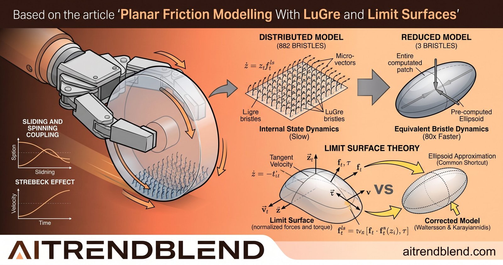
- The work combines the LuGre bristle friction model with limit surface theory to describe how sliding and spinning trade off during flat contact.
- A distributed version places a small friction element on every cell of the contact patch, which is accurate but slow, needing 882 internal state variables in the running example.
- A reduced version squeezes the same behaviour into three bristles and a pre computed limit surface, running around 80 times faster with only 3 state variables.
- The authors challenge a common shortcut, showing that the ellipsoid approximation of the limit surface misplaces the force for a given velocity more than the literature usually admits.
- An Elasto-Plastic extension stops the model from slowly drifting when it is shaken by oscillating loads below the slip threshold.
- Everything is validated in simulation against grasping and pushing style motions, with open source code released alongside the paper.
Why flat contact breaks the textbook friction model
Most engineers meet friction as a single number. Coulomb told us the force opposing motion is proportional to the normal load, and for a block sliding in a straight line that story holds up well enough. The problem runs deeper than it first appears once the contact is a patch rather than a point, and once the object is allowed to rotate while it slides.
Think about what a fingertip actually does when it holds a coin and lets it pivot. Every tiny area of the contact moves in a slightly different direction, because rotation gives each point its own velocity depending on where it sits relative to the center of rotation. Some parts of the patch drag one way while others drag another. The total friction is the sum over all of those little contributions, and the sum couples the straight line force to the twisting torque. Push harder tangentially and the object resists spinning less. Spin it and it slides more easily. One number cannot express that.
This coupling is exactly what matters for a robot doing fine manipulation. Gabriel Arslan Waltersson and Yiannis Karayiannidis frame the whole paper around it, and they choose two established ideas to build on rather than inventing a model from nothing. The first is the LuGre friction model, which handles the messy behaviour near zero velocity, the regime where an object is neither fully stuck nor fully sliding. The second is limit surface theory, which handles the geometry of how force and torque trade off across a patch. The contribution is welding the two together and then making the result cheap enough to run.
Background, the bristles under a sliding surface
The LuGre model has a physical picture behind it that is worth carrying in your head. Imagine the two surfaces in contact as two brushes pressed together. The bristles bend elastically before anything slips. That average bend is a hidden state, written \(z\), and the friction force depends on how far the bristles are deflected and how fast they are deflecting. Carlos Canudas de Wit and his coauthors introduced this idea in 1995 as an extension of the earlier Dahl model, and its strength is that it reproduces the Stribeck effect, the dip in friction as an object first breaks free and starts to move.
The amended LuGre model that the paper starts from lets the normal load vary over time, which matters for a gripper that is squeezing harder or softer. The bristle deflection rate is written as follows.
Here \(v\) is the relative velocity between the surfaces and \(\sigma_0\) is the bristle stiffness. The function \(g(v)\) encodes the Stribeck shape, blending the static friction coefficient \(\mu_S\) down toward the Coulomb value \(\mu_C\) as speed rises.
The friction force itself adds three pieces, a spring like term from the bristle deflection, a damping term from how fast the bristles are moving, and a plain viscous term that grows with speed.
All of that is one dimensional. It describes a block sliding along a line. The leap the paper makes is to carry this bristle machinery into two dimensions and spread it across a real contact area.
The limit surface, a map of force against torque
Limit surface theory came out of the robotics grasping community in the late 1980s, with Suh Goyal, Andy Ruina, and Jim Papadopoulos among the names most associated with it. Here is where it gets interesting. For a given contact patch under Coulomb friction, you can draw a closed surface in the space whose axes are the two tangential force components and the torque. Any motion of the object corresponds to a point on that surface, and the direction of motion is normal to the surface at that point. The surface is a complete map of every friction wrench the patch can produce.
The tangential forces and the torque that define this surface come from integrating the local friction over the patch.
The vector \({\rho}\) points from the center of pressure to each little area \(dA\), and \(p(x,y)\) is the pressure at that spot. Change the pressure distribution, from a uniform disc to a ring to a line, and you change the shape of the limit surface, which is why a soft fingertip and a hard edge behave so differently under the same load.
For years the practical move has been to skip the integral and approximate the limit surface as an ellipsoid. It is simple, it is quick, and it looks about right. The paper takes a harder look at that shortcut, and the verdict is one of its more useful results.
The comparison between the limit surface and the ellipsoid approximation is commonly depicted using plots that focus solely on the closest distance, which flatters the approximation and hides where it actually fails. Waltersson and Karayiannidis, on why the ellipsoid looks better than it is
Building the distributed model
The first concrete model in the paper is the distributed planar friction model. The idea is direct. Take the contact area, chop it into a grid of cells, and drop a full two dimensional LuGre element into each cell. Every cell has its own bristle deflection state, its own local velocity coming from the object motion, and its own slice of the pressure. Add up the forces and the torques from all the cells and you have the total friction wrench.
The two dimensional bristle rate couples the x and y directions through the magnitude of the velocity, which is the piece that makes the planar case different from two independent one dimensional models.
In the running example the authors use a circular contact of 10 mm radius under a 1 N load, discretized into a 21 by 21 grid. That grid is where the cost lives. Each cell carries state, and the running example ends up with 882 internal state variables that a solver has to track and update at every step. The accuracy is excellent, and the model handles awkward pressure patterns such as a gradient line or a non convex patch without special cases. What it does not have is speed.
The discretization has a rough edge
Chopping a smooth patch into square cells introduces an artifact. As the center of rotation drifts across the patch, the friction force jumps in small steps every time the rotation center crosses from one cell into the next. You can see it in the paper as a staircase in the force curves. The authors smooth this with a bilinear interpolation on the steady state friction, treating the four corners of the cell that holds the rotation center and blending between them. It is a small fix with a real payoff, because those steps would otherwise leak into whatever controller sits downstream.
The reduced model, three bristles instead of hundreds
This is the heart of the paper, and it is a nice piece of engineering. Rather than simulate every cell, the authors collapse the whole patch into a circular rim contact described by just three bristles. The coupling between those three bristles is governed by a pre computed limit surface, so the expensive integral over the patch is done once, offline, and stored.
The reduced force wrench is expressed through a twist velocity vector \(\mathbf{v} = [v_x\; v_y\; \omega]^T\) that carries both the linear and the angular motion of a frame at the center of pressure. A radius \(r\) sets the scale of the equivalent rim contact. Under the ellipsoid version, the mapping from scaled velocity to force wrench takes a clean form.
The diagonal matrix \(\mathbf{S}\) scales the last element into a torque based on the radius, and \(r\) can be pre calculated for a given surface from the pressure distribution. The whole point is that the shape of the patch is baked into a handful of constants ahead of time, so the online cost no longer depends on how many cells you would have needed.
How much does this save. In the paper’s own timing, simulating two seconds of a slip stick experiment with a circular patch takes the distributed model about 218 seconds and the reduced model about 3.5 seconds. For a 21 by 21 patch the speedup lands near 80 times. The reduced model carries 3 state variables where the distributed one carries 882. That is not a marginal tune up, it is the difference between a model you can run in a controller and one you cannot.
| Contact and pressure | Distributed model | Reduced model | Speed factor |
|---|---|---|---|
| Circle, load independent shape | 217.98 s | 3.47 s | about 63 times |
| Pressure exponent k of 2 | 237.06 s | 3.49 s | about 68 times |
| Pressure exponent k of 2 times load | 238.95 s | 70.23 s | about 3.4 times |
The last row is honest about a limit. When the shape of the contact patch itself changes with the normal load, the pre computed limit surface has to be recomputed as the load moves, and in that experiment the normal force updates at 100 Hz. The reduced model still wins, but the margin narrows sharply. It is a fair reminder that the trick depends on the geometry staying fixed enough to be cached.
Where the ellipsoid approximation goes wrong
The reduced model with a plain ellipsoid limit surface does not exactly reproduce the distributed model, and the paper is careful to show why rather than wave the gap away. Two surfaces can look almost identical in a plot of closest distance and still disagree badly about which velocity maps to which point. That correspondence between a given velocity and its location on the surface is what actually drives the simulated force, and it is where the ellipsoid slips.
A concrete failure case makes it vivid. For a gradient line contact, where the pressure is heavier at one end than the other, there exists a point where a pure rotation produces zero tangential force. The ellipsoid approximation always predicts zero tangential force for a pure rotation about the center of pressure. Those two points are not the same for a gradient line, because the tangential friction depends on the local pressure and the sign of the local velocity across the patch, while the center of pressure only depends on how the pressure is distributed. The ellipsoid, by construction, cannot tell them apart.
The fix is a limit surface correction. Instead of the ellipsoid, the authors pre compute the true normalized limit surface as a hash map indexed by spherical coordinates over the velocity directions, with bilinear interpolation inside each cell of the map. A scaled bristle deflection rate then follows that stored surface rather than the ellipsoid.
With this correction in place the reduced model tracks the distributed model closely across circular, square, line, gradient line, and non convex patches. A box plot in the paper compares the correction against the ellipsoid across all of those shapes, and the correction wins on every one, most dramatically on the gradient line where the ellipsoid struggles most.
Stopping the drift with Elasto-Plastic bristles
There is a known flaw in the plain LuGre model. Shake it with an oscillating tangential load that never crosses the threshold needed to make the object actually slip, and the model slowly creeps anyway. The object drifts across the table even though physically it should stay put. Pierre Dupont and colleagues diagnosed this years ago and proposed the Elasto-Plastic model for the one dimensional case, where bristle deflections below a breakaway threshold behave as a pure elastic spring and cannot accumulate into net motion.
The paper extends this idea to the planar case, which is not a simple copy because the deflection and the velocity are now vectors that can point in different directions. The authors use a cosine similarity between the unit velocity vector and the unit bristle deflection vector to decide how elastic the response should be, then blend smoothly from elastic to plastic as the deflection grows toward its maximum.
In the drift tests, a 1 kg disc of 0.05 m radius is driven by oscillating tangential loads, then by combined oscillating tangential and torsional loads, and finally by an oscillating normal load on top of a constant tangential pull. The plain planar LuGre model drifts in every case. The Elasto-Plastic extension removes the drift under the tangential and torsional loads and strongly reduces it under the oscillating normal load, where a small residual oscillation remains. The reduced model shows the same pattern, which is reassuring, because it means the cheap model did not lose the physics that motivated the fix.
Does it hold up on manipulation style motion
The most relevant test for robotics is the in hand slip stick experiment. A rectangular object of 0.15 by 0.08 m and 0.2 kg sits in a parallel gripper, and the normal force is switched on and off at 100 Hz while the object is allowed to slide and pivot. Two placements of the center of mass are tried, one that pivots and one that combines rotation and translation more evenly, and several pressure profiles are run through both.
Across these runs the reduced model follows the distributed model closely, tracking the object trajectory, the contact forces, and the torque with near identical outcomes. The numbers tell a consistent story. The cheap model is not a rough stand in, it is a faithful one, as long as the contact geometry is the kind that can be cached. That caveat is the honest boundary of the method, and the authors state it plainly rather than burying it.
For tasks where accurately modelling the slip stick regime is of critical importance, like controlled in hand sliding and manipulation, the reduced model offers an alternative to hybrid friction models and extends what has been developed for one degree of freedom to the planar case. From the paper’s conclusion
Honest limitations
A few real constraints sit around this work, and they matter for anyone thinking of using it. The validation is entirely in simulation. There is no physical rig with a real gripper and a force torque sensor confirming that the predicted wrenches match measured ones, and the authors themselves call for an accessible benchmark based on real world experiments as future work. Simulation against a finer simulation is a valid check on internal consistency, but it is not the same as contact with the physical world.
The caching that makes the reduced model fast assumes the contact shape stays fixed. When the pressure distribution changes with the normal load, as it does for a genuinely soft fingertip that spreads under pressure, the limit surface must be recomputed and much of the speed advantage fades, as the third row of the timing table shows. The method is strongest for contacts whose shape is stable even as the load varies.
There is also the modelling assumption of equal friction properties in all directions, which lets the authors sample only half of the velocity sphere when they build the limit surface map. Anisotropic contacts, such as a brushed or grooved surface that grips differently along and across the grain, fall outside what the pre computation handles as written. And the whole framework rests on Coulomb friction as the base for the limit surface, so materials that stray far from that assumption would need rework.
Reproducing the reduced model
The paper ships open source code in C plus plus for speed, but the clearest way to understand the reduced model is to build a small version of it and watch the bristle state evolve. The implementation below writes the reduced three bristle planar LuGre model as a differentiable module, which is a natural fit for robotics work that wants to place a friction model inside a learning or optimization loop. It uses the ellipsoid limit surface for clarity, integrates the bristle state with a simple explicit scheme, and includes a runnable smoke test on a driven velocity profile. The comments flag exactly where the ellipsoid would be swapped for the pre computed limit surface hash map from the paper.
# Reduced planar LuGre friction model with an ellipsoid limit surface.
# Educational reimplementation of the reduced model from Waltersson and
# Karayiannidis, "Planar Friction Modelling with LuGre Dynamics and Limit
# Surfaces" (arXiv:2308.01123). Written as a torch.nn.Module so the model
# is differentiable and can sit inside a learning or optimization loop.
# Note. The paper reports friction routines, not training losses. The
# "loss" functions here are simulation residuals for fitting or checking,
# not a claim that the original work trained a network.

import torch
import torch.nn as nn


class ReducedPlanarLuGre(nn.Module):
    """Three bristle planar LuGre friction with an ellipsoid limit surface.

    State vector z has three components, two tangential and one torsional.
    The twist velocity v = [vx, vy, omega] is expressed at the center of
    pressure. The radius r scales angular terms into an equivalent rim
    contact and is pre computed from the pressure distribution.
    """

    def __init__(self, mu_c=1.0, mu_s=1.2, v_s=1e-3, gamma=2.0,
                 sigma_0=1e6, sigma_1=8e2, sigma_2=0.2, radius=0.05):
        super().__init__()
        # Friction parameters, taken from Table I of the paper (p = 1).
        self.mu_c = mu_c            # Coulomb coefficient
        self.mu_s = mu_s            # static coefficient
        self.v_s = v_s              # Stribeck velocity
        self.gamma = gamma          # Stribeck exponent
        self.sigma_0 = sigma_0      # bristle stiffness
        self.sigma_1 = sigma_1      # bristle damping
        self.sigma_2 = sigma_2      # viscous friction
        self.r = radius             # equivalent rim radius
        # S maps the twist velocity into scaled units. The last element
        # turns angular velocity into an equivalent rim linear speed.
        self.register_buffer("S", torch.tensor([1.0, 1.0, radius]))

    def g(self, speed):
        """Stribeck function g(v). Blends static down to Coulomb friction."""
        stribeck = torch.exp(-(torch.abs(speed) / self.v_s) ** self.gamma)
        return self.mu_c + (self.mu_s - self.mu_c) * stribeck

    def steady_state_z(self, v_scaled):
        """Ellipsoid steady state bristle deflection for a scaled velocity.

        Swap this whole block for a lookup into the pre computed limit
        surface hash map h(r, v) to reproduce the corrected model from
        Section V-C of the paper.
        """
        speed = torch.linalg.norm(v_scaled) + 1e-12
        direction = v_scaled / speed
        return self.g(speed) * direction / self.sigma_0

    def bristle_rate(self, z, v):
        """Time derivative of the three bristle state, equation (25).

        z_dot = S v - z sigma_0 ||v_S|| / g(||v_S||). The ellipsoid limit
        surface enters through the scaling matrix S. Replace with the
        pre computed h(r, v) map for the corrected model.
        """
        v_scaled = self.S * v
        speed = torch.linalg.norm(v_scaled) + 1e-12
        return v_scaled - z * (self.sigma_0 * speed / self.g(speed))

    def force(self, z, z_dot, v, f_n):
        """Force wrench at the center of pressure, equation (26).

        Returns [fx, fy, tau] scaled by the normal load f_n.
        U carries the viscous friction, with the angular term scaled by r.
        """
        U = torch.tensor([1.0, 1.0, self.r], device=z.device)
        wrench = -(self.sigma_0 * z + self.sigma_1 * z_dot
                   + self.sigma_2 * U * (self.S * v)) * f_n
        return wrench

    def step(self, z, v, f_n, dt):
        """One stable integration step, returns the new state and the wrench.

        The bristle stiffness sigma_0 is large, so the deflection dynamics
        are stiff. The paper uses a stiff solver (LSODA). Here a semi
        implicit update keeps the linear decay term stable at a plain time
        step, which is enough for illustration and for gradients.
        """
        v_scaled = self.S * v
        speed = torch.linalg.norm(v_scaled) + 1e-12
        decay = self.sigma_0 * speed / self.g(speed)
        z_new = (z + dt * v_scaled) / (1.0 + dt * decay)
        z_dot = (z_new - z) / dt
        wrench = self.force(z_new, z_dot, v, f_n)
        return z_new, wrench

    def forward(self, z, v, f_n):
        """One evaluation. Returns the bristle rate and the force wrench."""
        z_dot = self.bristle_rate(z, v)
        wrench = self.force(z, z_dot, v, f_n)
        return z_dot, wrench


def simulate(model, v_profile, f_n, dt=1e-4):
    """Semi implicit roll out over a velocity profile.

    v_profile is a tensor of shape [T, 3] holding the twist velocity at
    each step. Returns the force wrench history of shape [T, 3].
    """
    z = torch.zeros(3, dtype=v_profile.dtype)
    history = []
    for t in range(v_profile.shape[0]):
        z, wrench = model.step(z, v_profile[t], f_n, dt)
        history.append(wrench)
    return torch.stack(history)


def tracking_loss(model, v_profile, reference, f_n, dt=1e-4):
    """Mean squared residual between predicted and reference wrenches.

    Use this to fit parameters against a distributed model roll out, the
    kind of validation the paper runs in Figures 17 and 19 to 21.
    """
    predicted = simulate(model, v_profile, f_n, dt)
    return torch.mean((predicted - reference) ** 2)


def smoke_test():
    """Runnable check on a driven velocity profile with dummy data."""
    torch.manual_seed(0)
    model = ReducedPlanarLuGre()

    steps = 2000
    time = torch.linspace(0.0, 0.2, steps).unsqueeze(1)
    # Drive a slide in x that ramps up, plus a gentle spin, to excite
    # the coupling between tangential force and torque.
    vx = 0.01 * torch.sin(2 * torch.pi * 5 * time)
    vy = torch.zeros_like(time)
    omega = 0.5 * torch.sin(2 * torch.pi * 3 * time)
    v_profile = torch.cat([vx, vy, omega], dim=1)

    f_n = torch.tensor(1.0)
    wrench = simulate(model, v_profile, f_n)

    assert wrench.shape == (steps, 3), "unexpected output shape"
    assert torch.isfinite(wrench).all(), "non finite forces produced"
    fx, fy, tau = wrench[-1]
    print("final wrench  fx {:.4f} N  fy {:.4f} N  tau {:.5f} Nm".format(
        fx.item(), fy.item(), tau.item()))
    print("peak tangential force {:.4f} N".format(
        torch.linalg.norm(wrench[:, :2], dim=1).max().item()))
    print("smoke test passed")


if __name__ == "__main__":
    smoke_test()
The one place to be careful is the steady state deflection. The version above uses the ellipsoid form for readability, which is the very approximation the paper improves on. To reproduce the corrected behaviour you replace the body of steady_state_z with a lookup into the pre computed limit surface, indexed by the two spherical angles that describe the velocity direction, exactly as Section V of the paper lays out. The rest of the module stays the same, which is a fair illustration of how modular the correction is.
What this changes for robot manipulation
Step back from the equations and the value is a practical one. Simulators such as the physics engines behind modern robot learning need friction models that are both faithful and fast. A model that needs 882 state variables per contact will not survive a scene with many contacts updating hundreds of times a second. A model with 3 state variables per contact that still captures the slip stick coupling might. That is the gap the reduced model aims at.
The honest read is that this is a strong simulation result waiting for physical validation. The coupling between sliding and spinning is real, the critique of the ellipsoid approximation is well argued and useful on its own, and the Elasto-Plastic drift fix addresses a genuine failure mode. What remains is the step from a finer simulation to a force torque sensor on a real gripper, and the authors are upfront that this is where the work should go next. For a researcher building contact rich manipulation, the reduced model is worth a look, and the open source release makes trying it cheap.
If you are mapping the broader landscape of robot autonomy, this friction work sits alongside other planning and perception problems covered on the site, from how robot path planning has evolved to how language models are learning to reason about 3D scenes. Contact modelling is the layer where a robot finally touches the world, and getting it right is what turns a plan into a successful grasp. You can browse the full set of related work through the robotics and autonomous systems pillar.
Conclusion
The core achievement of this paper is a planar friction model that respects the coupling between sliding and spinning without paying the full cost of simulating every point of the contact. The distributed version establishes the ground truth by spreading two dimensional LuGre elements across the patch, and the reduced version distills that behaviour into three bristles and a cached limit surface that runs around 80 times faster while carrying only 3 state variables. That is the headline, and it is a real one for anyone who needs friction inside a control or simulation loop.
The conceptual shift underneath it is a willingness to question a comfortable approximation. The ellipsoid limit surface has been the default for years because it is cheap and photogenic in the usual plots. By showing that it misplaces the friction force for asymmetric patches, and by offering a pre computed correction that fixes the problem without much added cost, the authors improve the accuracy of a tool that a lot of downstream work quietly depends on. That kind of careful correction tends to matter more over time than a flashy new architecture.
The ideas here also travel. Tire friction, walking robot foot contact, pushing and sliding of objects on a table, and the fine control of a grasped part all live in the same planar friction world, and the same LuGre plus limit surface recipe applies with different pressure distributions plugged in. The Elasto-Plastic extension carries over too, wherever oscillating loads threaten to make a model drift when it should hold still.
The remaining limitations are worth repeating rather than glossing over. The validation is in simulation, the caching assumes a stable contact shape, and the framework assumes isotropic Coulomb friction as its base. None of these sink the contribution, but they mark the edges of where it can be trusted today. Future work that puts the model on a physical gripper with a force torque sensor, and that builds a shared benchmark from real measurements, would turn a promising simulation result into a validated tool.
For now the paper does something quietly valuable. It takes two well understood ideas, joins them cleanly, makes the result fast, and tells you honestly where the joins are weakest. In a field that often oversells, that restraint is its own kind of contribution.
Frequently asked questions
What is planar friction and why does it need a special model?
Planar friction is the friction between two flat surfaces that can both slide and rotate against each other at the same time. A single Coulomb friction number cannot describe it, because the sliding force and the twisting torque are coupled. Pushing harder tangentially makes the object easier to spin, and spinning it makes it easier to slide. Robotic grasping and pushing live in this regime, which is why a dedicated planar model is worth the effort.
What does the LuGre model add over classic Coulomb friction?
The LuGre model treats the contact as microscopic bristles that bend before anything slips, using a hidden state for the average bend. This lets it capture the behaviour near zero velocity, the sticky regime where an object is neither fully stuck nor fully sliding, and it reproduces the Stribeck effect where friction dips as an object first breaks free. Classic Coulomb friction has none of that detail.
Why is the reduced model so much faster than the distributed one?
The distributed model places a friction element on every cell of the contact patch, which in the running example means 882 internal state variables a solver must track. The reduced model collapses the patch into three bristles coupled through a limit surface that is computed once and stored. That leaves only 3 state variables, and it runs around 80 times faster for a 21 by 21 contact while matching the distributed forces closely.
What is wrong with the ellipsoid approximation of the limit surface?
The ellipsoid is cheap and it looks accurate in plots that show only the closest distance between surfaces. The problem is the correspondence between a velocity and its location on the surface, which drives the simulated force. For asymmetric patches such as a gradient line contact, the ellipsoid places the force in the wrong spot, for example predicting zero tangential force for a pure rotation when the real patch produces a force. The paper replaces it with a pre computed limit surface to fix this.
What does the Elasto-Plastic extension fix?
The plain LuGre model drifts when it is shaken by oscillating loads that stay below the level needed to make an object actually slip. The object creeps across the surface when it should stay put. The Elasto-Plastic extension makes small bristle deflections behave as a pure elastic spring so they cannot build into net motion, which removes the drift under oscillating tangential and torsional loads and strongly reduces it under an oscillating normal load.
Has this model been tested on a real robot?
No. The validation in the paper is entirely in simulation, where the fast reduced model is checked against a finer distributed model. The authors call for an accessible benchmark based on real world experiments as future work. The results are a strong internal consistency check and a useful critique of common approximations, but confirmation against a physical gripper with a force torque sensor is still open.
Go to the source
Read the full paper and run the authors’ own implementation.
Read the paper on arXiv Open the code on GitHubSource paper. Gabriel Arslan Waltersson and Yiannis Karayiannidis, “Planar Friction Modelling with LuGre Dynamics and Limit Surfaces,” accepted to IEEE Transactions on Robotics, 2024. Preprint at arXiv:2308.01123. Code at github.com/Gabrieleenx/FrictionModelling.
This analysis is based on the published paper and an independent evaluation of its claims.