
Key points
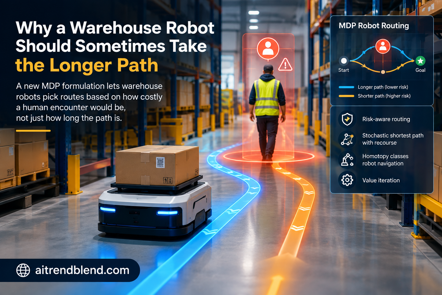
- The paper reframes robot routing as a decision problem where the true cost of a corridor, meaning the delay from a human encounter, only becomes known once the robot stands at the intersection that opens onto it.
- Instead of tracking every possible position of every person, which would blow up into more than ten to the seventeenth states in a fifty corridor warehouse, the authors compress the problem into a Markov decision process whose state count grows only linearly with the number of intersections.
- They identify and prove a genuine failure mode. Because a Markov decision process forgets what it already observed, a naive version of this approach can send the robot into an endless loop chasing a better observation that will never come.
- Their fix updates the policy online the moment a person is spotted, and they prove this stops the loop and still guarantees the robot reaches the goal.
- Real robot trials on a Robotnik XL Steel platform measured the actual time penalty of passing a person in a narrow versus a wide corridor, and the numbers back up the model’s core assumption that width matters as much as length.
The problem with routing on expected length alone
Most indoor robots plan the way GPS plans a car trip. Build a map, assign each segment a cost such as distance, then run a shortest path search. That works well when the map does not change. It works far less well in a warehouse, hospital or factory floor, where people move through the same corridors the robot needs and where slowing down or replanning around a person is not optional. Safety rules such as ISO 15066 require the robot to yield, and yielding costs time.
The authors are careful about what they mean by risk here. They are not talking about collision probability, which is the usual meaning in motion planning papers. They define risk the way a project manager would, as an uncertain event that degrades the chance of finishing a task well. A person blocking a corridor is not dangerous in the collision sense if the robot simply stops and waits, but it is still a risk because it burns time and forces a stressful close encounter. The paper’s cost function reflects that framing directly. It adds path length to a penalty that only appears when an obstruction is actually met, and the size of that penalty depends on how easy the corridor is to replan around.
This distinction matters because it changes what counts as a good route. A narrow aisle with no room to step aside turns any encounter into a full stop and a slow squeeze past, which is expensive under this metric even if nobody is ever actually detected there. A wide corridor lets the robot glide around a person without much loss, so an occasional detour into it is cheap insurance. Classic shortest path planning cannot represent that tradeoff at all, because it has no concept of what happens if a person shows up.
A warehouse operator tuning a fleet’s routing logic usually has one lever, an occupancy penalty added to blocked cells. This paper argues that the penalty needs a second dimension, how expensive an encounter is to recover from in that specific location, not just whether one might happen there.
Borrowing from a decades old traveler and giving it a memory problem
The routing setup here descends from a classic puzzle called the Canadian traveler problem, first posed by Bar Noy and Schieber in 1991, where a traveler discovers that a road is blocked only once they arrive at its start. The paper works with a specific branch of that problem called stochastic shortest path with recourse, introduced by Polychronopoulos and Tsitsiklis in 1996, in which every road stays passable but its true cost is revealed only when the traveler reaches it. Warehouse corridors fit this second version better than the classic one, since a robot can always squeeze past a person eventually, it just costs more to do so.
Prior robotics work in this space tends to split into two camps. One camp treats risk purely as collision probability and folds it into a modified A star search, as Primatesta, Guglieri and Rizzo did for drone path planning around urban hazards. The other camp, closer in spirit to this paper, is Chung, Smith, Skeele and Hollinger’s risk aware graph search, which models edge costs as continuous Gaussian variables that get revealed with recourse. The Pisa group builds directly against that second line of work, and they are candid about the tradeoff. Gaussian edge costs make expensive events like a human encounter hard to represent well, since a Gaussian assumes a smooth spread rather than a discrete jump from empty to occupied. Their model instead uses discrete probabilities tied to whether a person is present at all, which maps much more naturally onto what a robot’s sensors actually report.
The harder problem the authors take on is the state explosion that comes from trying to track where every person in the building might be. A full partially observable Markov decision process over fifty corridors and twenty people would need on the order of ten to the seventeenth states just to represent the possible ways those twenty people could be distributed. Nobody is solving that at runtime. The paper’s central engineering move is to stop tracking people directly and instead track observations, meaning the zero or one signal the robot’s sensors return for each nearby corridor. That single substitution turns an intractable partially observable problem into a fully observable Markov decision process whose size scales with the number of intersections, not the number of people or where they might be standing.
How the state actually gets built
Each state in the model bundles three things. The node the robot currently occupies, the node it just came from, and a tuple of zero or one flags for every other corridor branching off that intersection. A person is flagged as detected only if they sit in the portion of the corridor the robot can actually see from where it stands, which the paper computes geometrically by checking line of sight against the static obstacle map. If an intersection has three outgoing corridors and the robot arrived along one of them, the remaining two corridors each contribute a binary observation, giving four possible states for that arrival direction alone.
Two design choices keep this compact. First, the robot is barred from ever backtracking onto the corridor it just arrived from at a decision point. Second, the goal collapses into a single absorbing state regardless of how the robot got there. Together these choices give a state count that the authors show grows as roughly the number of intersections times a term that is exponential only in the maximum number of corridors meeting at any single intersection, not in the size of the whole map. For the realistic warehouse layouts they tested, where intersections rarely have more than four or five branches, this stays entirely tractable even as the map grows large.
Actions are just the choice of which outgoing corridor to take next, excluding the one the robot arrived from. Transition probabilities capture something specific and a little subtle, which is the chance of making a particular pair of observations at the next intersection, computed by treating each outgoing corridor’s occupancy as independent. Rewards, or in this case costs, come from the expected length of the chosen corridor plus a penalty scaled by how many people are likely to be encountered given whatever was just observed.
That severity coefficient deserves a closer look, because it is doing most of the interesting work in the model. The authors define it as a simple piecewise linear function of corridor width relative to robot width, capped at both ends. A corridor wide enough to let the robot pass comfortably gets a severity of zero. A corridor barely wider than the robot itself gets the maximum penalty, since any encounter there forces a full stop and a careful, slow maneuver. Everything in between scales linearly. This is a modeling simplification, and the authors are upfront that it is a starting point rather than a measured physical law, but it gives the framework something concrete to calibrate against real corridor geometry pulled straight from a generalized Voronoi diagram of the floor plan.
The loop nobody wanted, and the fix that closes it
Here is where the paper earns its place beyond a routine application of value iteration. A Markov decision process is memoryless by definition. It does not remember what it saw two steps ago on the same corridor. That is normally a convenience, but the authors show it becomes a genuine hazard in this setting. Consider a robot standing at an intersection where the only path to the goal is blocked by a person. If the policy computed offline decides that looping around through several other intersections and coming back is cheaper than crossing the occupied corridor, in the hope of getting a fresh, better observation on the return trip, the robot will do exactly that. If the person never moves, because they are working at a fixed station rather than walking through, that hopeful loop never pays off and the robot cycles forever.
The paper proves this rigorously rather than just demonstrating it anecdotally. Lemma 1 spells out three conditions that all have to hold for a loop to look attractive to the planner, including that the loop must have a real chance of flipping the bad observation back to a good one. Corollary 1 then shows that if the obstruction is static, that flip probability is zero, which means the offline policy still thinks the loop is worthwhile even though it can never actually deliver on that promise. That mismatch between what the memoryless model believes and what is physically true is the whole bug, laid out with a formal proof rather than hand waving.
Their fix is refreshingly simple given how carefully the failure mode was diagnosed. The moment the robot detects a person on a corridor, the system locks that corridor’s occupancy probability to one for the rest of the trip and immediately resolves the Markov decision process with that update baked in. This does two things at once. It removes the incentive for the planner to loop back hoping for a different reading, since the model now treats that reading as fixed, and it produces a fresh, locally correct policy for whatever remains of the trip. Theorem 1 proves that this sequence of local replans contains no infinite loops and reaches the goal with probability one, since each detection permanently shrinks the space of edges the planner is still uncertain about, and there are only finitely many edges to become certain about.
Locking a corridor to occupied for the rest of the trip is a conservative assumption. If a person only paused briefly and then moved on, the robot will keep avoiding that corridor even after it clears, which can slightly overstate cost in the offline plan. The authors accept this cost explicitly because the alternative, letting the planner hope for a better reading later, is what causes the infinite loop in the first place.
What happened when they tested it against A star, a smarter A star, and a dedicated risk search algorithm
The evaluation runs across three warehouse layouts of increasing size, plus a real robot deployment to ground the severity numbers in physical time measurements rather than assumptions. The comparisons are against plain A star on expected cost, a modified A star that replans every time it reaches a node with fresh information but is still allowed to backtrack, and the risk aware graph search algorithm from Chung and colleagues, adapted from continuous Gaussian costs to the paper’s discrete occupancy model.
| Approach | How it decides | Main limitation the paper reports |
|---|---|---|
| Plain A star on expected cost | Commits to one static path computed before departure | Never adapts once a person is spotted, consistently the most costly in simulation |
| Modified A star | Replans locally at each node using the freshest observation | Sometimes sticks with a bad first choice because it undervalues how many further replanning chances a different first move would open up |
| Risk aware graph search | Tracks nondominated candidate paths and updates which one looks best as it moves | Its initial search step gets very expensive on large maps, and a looser threshold setting only ever rediscovers the plain A star path |
| This paper’s MDP | Precomputes a full policy over observation states, then patches it locally on detection | Can slightly underestimate cost for static obstacles due to the loop assumption the online fix has to override |
On the smallest warehouse map, with eight nodes and a total of seventy seven states, the differences are already visible. When the severity of an encounter is set high, the proposed method consistently steers the robot down a central, wider corridor rather than the geometrically shorter path along the wall, and this choice lowers average cost across ten thousand simulated human configurations. The gap widens on the medium sized map with one hundred forty nine states, where the modified A star algorithm sometimes refuses to reroute even after spotting a person, because it underestimates how much better the alternative route’s own replanning options are further down the line. A paired permutation test across scenarios puts the improvement over the baselines at a statistically significant level, generally with a p value below 0.0008 wherever the new method actually outperforms the alternative.
The risk aware graph search comparison is the most nuanced result in the paper, and the authors do not oversell their own method here. On the medium map, that algorithm occasionally edges out the proposed approach because it is willing to backtrack to a previous decision point if conditions change, a move the MDP formulation deliberately forbids to avoid the looping problem described earlier. Where the new method wins decisively is scale. On the largest test map, with one hundred fifty seven nodes and nearly twenty five hundred states, the risk aware graph search algorithm’s initial planning sweep becomes computationally expensive enough to be impractical, since it has to propagate full discrete cost distributions across every candidate path rather than the cheap mean and variance updates a Gaussian model would allow. The proposed method, by contrast, solves the whole warehouse in a fraction of a second for the value iteration step itself.
Grounding the model in an actual robot
The most convincing part of the paper for a skeptical reader is probably the smallest section, tucked near the end. The team ran physical trials with a Robotnik XL Steel robot equipped with two SICK lidar units, using an obstacle detector package to pick out human sized objects and a modified TEB local planner that slows the robot down as a person gets closer. They measured how much extra time a real encounter cost in a narrow corridor around two point two five meters wide versus a wider one around three point seven five meters wide, both roughly seven meters long.
The narrow corridor added noticeably more delay on average than the wide one, which is exactly the assumption the severity coefficient is built on. But the more interesting finding is buried in the variance. Both distributions of added delay were wide and clearly not normal, because in some runs the robot got temporarily stuck negotiating space with the person, especially in the narrow corridor, and needed far longer than the median case to get past. That is a useful, honest data point for anyone trying to apply this kind of model in practice. A fixed severity number is a simplification of something that in reality depends heavily on how a specific person chooses to move out of the way.
Where this still falls short
The authors are explicit about several open edges rather than papering over them. The severity coefficient is a linear function of corridor width chosen for tractability, not derived from the real world delay data they collected, and their own experiments show that real delays have heavy tails the model does not capture. The independence assumption between corridors, needed to keep the transition tensor computation cheap, means the model cannot represent a person walking from one visible corridor into another, since each corridor’s occupancy is treated as its own coin flip. Star shaped intersections with many branches, while rare in real warehouses, would blow the state count up exponentially in the branching factor, a limitation the authors flag directly with a small worked example. And the online loop fix, while proven correct, achieves that correctness by permanently writing off any corridor where a person was ever spotted, which can leave the robot avoiding a corridor for the rest of its trip even after that person has long since moved along.
Broader implications for fleet routing
The framing here is more useful than the specific numbers, and that is probably the right way to read most papers in this space. Warehouse and hospital fleets already collect the kind of statistical information this model wants, corridor traffic patterns, typical dwell times, sensor visibility from each junction. What most fleets lack is a principled way to turn that data into a route choice that accounts for what happens after an encounter, not just the chance one occurs. This paper offers exactly that missing piece, expressed as a Markov decision process compact enough to solve on the fly and precise enough to prove properties about, such as the loop elimination guarantee that most heuristic routing systems simply cannot offer.
It is also a useful case study in how much mileage comes from choosing the right state representation before reaching for a bigger model. The naive instinct when uncertainty about human positions gets complicated is to reach for a partially observable Markov decision process and accept the computational cost. This paper’s real contribution is showing that swapping hidden human positions for observable sensor readings turns an intractable problem into one that scales cleanly, without giving up the ability to reason about replanning value, corridor visibility, and encounter severity together.
Conclusion
The core achievement of this work is a routing model that treats a human encounter as something with a cost that depends on where it happens, not merely whether it happens, and that folds this into a decision process small enough to solve for warehouses with hundreds of intersections. That single shift, from tracking people to tracking observations, is what makes the whole approach practical rather than a theoretical exercise confined to toy graphs.
The more conceptually interesting move is the honest reckoning with the model’s own blind spot. Plenty of papers propose a Markov decision process for a robotics problem and stop there. This one goes further, proves exactly when the memoryless assumption breaks down into an infinite loop, and then engineers a specific, provably correct patch rather than papering over the issue with a heuristic timeout or a hard coded step limit.
The underlying idea, replacing a hard to track hidden variable with the observable signal a real sensor would actually produce, is not specific to robots dodging people in corridors. Anywhere a planning problem has partial observability driven by a large hidden state space, from ride hailing dispatch reasoning about passenger demand to drone delivery reasoning about weather cells, the same compression trick is worth trying before reaching for a full partially observable solver.
The honest limitations are real and worth repeating rather than glossing over. The severity model is a starting approximation, the independence assumption between corridors will not hold in every layout, and star shaped intersections remain a genuine scaling weakness. None of that undoes the paper’s central contribution, but it does mean a team adopting this approach should expect to spend real effort calibrating severity coefficients against their own facility’s data rather than trusting the paper’s illustrative numbers directly.
What sticks with me most is the small physical experiment near the end. It would have been easy to publish the theory and simulation results alone, since the math stands on its own. Choosing to also measure real delay distributions on an actual robot, and then honestly reporting that those distributions are messier than the model assumes, is the kind of detail that separates a paper meant to be cited from one meant to be used.
Frequently asked questions
What is risk aware routing in this context
It means choosing a path for a robot based on the expected cost of the whole trip, including a penalty for any human encounter, rather than choosing the path with the shortest expected length alone.
How is this different from a partially observable Markov decision process
A fully partially observable formulation would try to track the possible locations of every person in the building, which becomes computationally impossible even for a modest warehouse. This paper’s Markov decision process instead tracks only the robot’s own observations at each intersection, which keeps the state space linear in the number of intersections.
Why can the offline policy get stuck in a loop
Because a Markov decision process has no memory of past observations, it can be tricked into believing that looping back through several intersections offers a real chance at a better reading on a corridor it already saw was blocked. If the obstruction is a person standing still rather than passing through, that better reading never comes, and the robot would cycle forever without the online fix.
Does this method beat every existing algorithm in every scenario
No, and the authors say so directly. The risk aware graph search algorithm from prior work occasionally produces a slightly cheaper path on medium sized maps because it allows backtracking that this method deliberately forbids. Where this method wins clearly is computational scalability on large maps, where the alternative’s planning sweep becomes impractically slow.
How was the severity of an encounter measured
The paper defines severity mainly as a function of corridor width relative to robot width, then separately validated the underlying assumption with physical trials on a real robot, measuring how much extra time an encounter added in a narrow corridor versus a wide one.
Could this run on a warehouse fleet today
The computational requirements look modest enough for real deployment, with policy computation and online updates measured in a fraction of a second on standard hardware even for a large map. The harder practical step is estimating the human presence and visibility parameters the model needs from real facility data rather than the paper’s illustrative distributions.
Read the source
The full paper, published in IEEE Transactions on Robotics, volume 42, 2026, includes the complete proofs, all three test maps, and the physical robot trial data referenced above.
Reference implementation, a torch based value iteration solver
The paper’s own experiments were run with a Python MDP toolbox rather than a neural network, since the method is a classical value iteration solver, not a trained model. The implementation below follows the paper’s state definition, transition tensor construction and reward computation closely, using torch tensors so the Bellman backup runs as a batched operation rather than a nested loop. It builds a small three way intersection, one narrow leg and one wide leg leading to a shared goal, and confirms the learned policy actually prefers the wide leg once it detects a person on the narrow one, which is the qualitative behavior the paper argues for throughout.
# Risk aware routing, reimplemented from Stracca, Grioli, Pallottino
# and Salaris, IEEE Transactions on Robotics, 2026.
# States bundle the current node, the predecessor node, and the
# observation made on every other outgoing corridor, following
# equation 8 of the paper. This keeps the state count linear in
# the number of intersections instead of exponential in the number
# of people that might be present.

import math
import torch

torch.manual_seed(0)


class HomotopyGraph:
    """A directed graph over decision points. Each edge stores a
    physical length and a corridor width, feeding the severity
    coefficient from equation 15 in the paper."""

    def __init__(self):
        self.nodes = []
        self.edges = {}

    def add_edge(self, u, v, length, width):
        for node in (u, v):
            if node not in self.nodes:
                self.nodes.append(node)
        self.edges[(u, v)] = {"length": length, "width": width}

    def out_edges(self, node):
        return [e for e in self.edges if e[0] == node]


def severity_coefficient(width, robot_width, k1=12.5, k2=62.5, k3=50.0):
    """Equation 15. Narrow corridors get a high penalty, wide ones
    get none."""
    raw = -k1 * (width - robot_width) + k2
    return max(0.0, min(raw, k3))


def binomial_person_count_pmf(n_mean, n_max):
    """Equation 16. Probability of exactly n people in the whole
    environment, modeled as a binomial trial over n_max slots."""
    p = n_mean / n_max
    pmf = torch.zeros(n_max + 1)
    for n in range(n_max + 1):
        pmf[n] = math.comb(n_max, n) * (p ** n) * ((1 - p) ** (n_max - n))
    return pmf


class RiskAwareRoutingMDP:
    """Builds S, A, P, R for a homotopy class graph and solves the
    resulting stochastic shortest path with recourse through value
    iteration, following Section IV and Section V of the paper."""

    def __init__(self, graph, goal, robot_width, n_mean, n_max, gamma=0.9999):
        self.graph = graph
        self.goal = goal
        self.robot_width = robot_width
        self.n_max = n_max
        self.gamma = gamma
        self.person_pmf = binomial_person_count_pmf(n_mean, n_max)
        self._compute_static_edge_properties()
        self._build_state_space()
        self._build_tensors()

    def _compute_static_edge_properties(self):
        total_length = sum(e["length"] for e in self.graph.edges.values())
        for edge, props in self.graph.edges.items():
            props["ph"] = props["length"] / total_length  # equation 13
            props["pv"] = 1.0
            props["cp"] = severity_coefficient(props["width"], self.robot_width)

    def _person_count_given_observation(self, ph, pv, obs):
        """Equations 17 to 19, returning p(k given obs) over k people
        truly present in this corridor."""
        n_max = self.n_max
        k_range = torch.arange(n_max + 1)
        p_k = torch.zeros(n_max + 1)
        for n in range(n_max + 1):
            if self.person_pmf[n] == 0:
                continue
            binom = torch.tensor([math.comb(n, k) if k <= n else 0.0
                                   for k in range(n_max + 1)])
            p_k += self.person_pmf[n] * binom * (ph ** k_range) * \
                   ((1 - ph) ** (n - k_range).clamp(min=0))

        p_obs_given_k = torch.zeros(n_max + 1)
        p_obs_given_k[0] = 1.0 if obs == 0 else 0.0
        for k in range(1, n_max + 1):
            p_see_none = (1 - pv) ** k
            p_obs_given_k[k] = p_see_none if obs == 0 else 1 - p_see_none

        p_obs = torch.sum(p_k * p_obs_given_k)
        if p_obs <= 1e-12:
            return torch.zeros(n_max + 1), p_obs
        return p_k * p_obs_given_k / p_obs, p_obs

    def _expected_edge_cost(self, edge, obs):
        """Equation 12, restricted to the static people model."""
        props = self.graph.edges[edge]
        p_k_given_obs, p_obs = self._person_count_given_observation(
            props["ph"], props["pv"], obs)
        k_range = torch.arange(self.n_max + 1)
        penalty = torch.sum(p_k_given_obs * k_range) * props["cp"]
        return props["length"] + penalty.item(), p_obs.item()

    def _build_state_space(self):
        """Equation 8. Every state is node, predecessor, observation
        tuple on the other outgoing edges. The goal collapses to
        one absorbing state."""
        self.states, self.state_index = [], {}
        for node in self.graph.nodes:
            if node == self.goal:
                continue
            out = self.graph.out_edges(node)
            preds = sorted({u for (u, v) in self.graph.edges if v == node}) or [None]
            for pred in preds:
                remaining = [e for e in out if e[1] != pred]
                if not remaining:
                    continue
                for bits in range(2 ** len(remaining)):
                    obs = tuple((bits >> i) & 1 for i in range(len(remaining)))
                    state = (node, pred, obs, tuple(remaining))
                    self.state_index[state] = len(self.states)
                    self.states.append(state)
        self.goal_state = (self.goal, None, (), ())
        self.state_index[self.goal_state] = len(self.states)
        self.states.append(self.goal_state)
        self.n_states = len(self.states)
        self.n_actions = max((len(s[3]) for s in self.states
                               if s != self.goal_state), default=1)

    def _observation_prob(self, edge, obs_value):
        props = self.graph.edges[edge]
        _, p_obs = self._person_count_given_observation(
            props["ph"], props["pv"], obs_value)
        return p_obs

    def _build_tensors(self):
        """Algorithm 1. Builds the transition tensor P and reward
        matrix R described in Section IV."""
        n_s, n_a = self.n_states, self.n_actions
        P = torch.zeros(n_a, n_s, n_s)
        R = torch.zeros(n_s, n_a)

        for state in self.states:
            si = self.state_index[state]
            if state == self.goal_state:
                P[:, si, si] = 1.0
                continue
            node, pred, obs_tuple, remaining = state
            for a, edge in enumerate(remaining):
                next_node = edge[1]
                cost, _ = self._expected_edge_cost(edge, obs_tuple[a])
                R[si, a] = -cost
                if next_node == self.goal:
                    P[a, si, self.state_index[self.goal_state]] = 1.0
                    continue
                next_out = [e for e in self.graph.out_edges(next_node) if e[1] != node]
                if not next_out:
                    P[a, si, self.state_index[self.goal_state]] = 1.0
                    continue
                for bits in range(2 ** len(next_out)):
                    next_obs = tuple((bits >> i) & 1 for i in range(len(next_out)))
                    prob = 1.0
                    for j, ne in enumerate(next_out):
                        p_one = self._observation_prob(ne, 1)
                        prob *= p_one if next_obs[j] == 1 else (1 - p_one)
                    sj = self.state_index[(next_node, node, next_obs, tuple(next_out))]
                    P[a, si, sj] += prob
            for a in range(len(remaining), n_a):
                P[a, si, si] = 1.0
                R[si, a] = -1e6
        self.P, self.R = P, R

    def solve(self, n_iterations=500, tol=1e-6):
        """Value iteration on the Bellman equation from Section IV."""
        V = torch.zeros(self.n_states)
        for _ in range(n_iterations):
            Q = self.R + self.gamma * torch.einsum("ass,s->sa", self.P, V)
            V_new, policy = torch.max(Q, dim=1)
            if torch.max(torch.abs(V_new - V)) < tol:
                V, self.policy = V_new, policy
                break
            V = V_new
        else:
            self.policy = policy
        self.V = V
        return V, self.policy


def build_toy_intersection(robot_width=0.8):
    """A three way intersection with one narrow leg and one wide
    leg leading to the goal, used as the smoke test graph."""
    g = HomotopyGraph()
    g.add_edge("S", "A", length=8.0, width=3.5)
    g.add_edge("A", "B", length=6.0, width=1.2)   # narrow, high severity
    g.add_edge("A", "C", length=9.0, width=3.0)   # wide, low severity
    g.add_edge("B", "G", length=4.0, width=1.2)
    g.add_edge("C", "G", length=4.0, width=3.0)
    return g


def run_smoke_test():
    graph = build_toy_intersection()
    mdp = RiskAwareRoutingMDP(graph=graph, goal="G", robot_width=0.8,
                               n_mean=3, n_max=8)

    print(f"Number of states  : {mdp.n_states}")
    print(f"Number of actions : {mdp.n_actions}")

    row_sums = mdp.P.sum(dim=2)
    assert torch.allclose(row_sums, torch.ones_like(row_sums), atol=1e-4), \
        "transition tensor rows must sum to one for every state and action"

    V, policy = mdp.solve()
    assert torch.isfinite(V).all(), "value function must stay finite"

    node_a_states = [s for s in mdp.states if s[0] == "A"]
    print("Policy at node A, split by observation on each leg")
    for state in node_a_states:
        si = mdp.state_index[state]
        chosen = state[3][policy[si].item()]
        print(f"  observed {state[2]} on legs {state[3]} -> take {chosen}")

    print("Smoke test passed.")


if __name__ == "__main__":
    run_smoke_test()
Running this against the small three way graph produces eleven states and two actions, confirms every row of the transition tensor sums to one as a sanity check on Algorithm 1, and prints a policy table showing the robot switching from the narrow leg to the wide leg the moment the narrow leg reports a detection, exactly the qualitative behavior the paper spends its middle sections proving is correct and loop free.
Stracca, E., Grioli, G., Pallottino, L. and Salaris, P. Risk aware routing for a robot in a shared dynamic environment. IEEE Transactions on Robotics, volume 42, 2026, pages 1048 to 1067. DOI 10.1109/TRO.2026.3658295.