
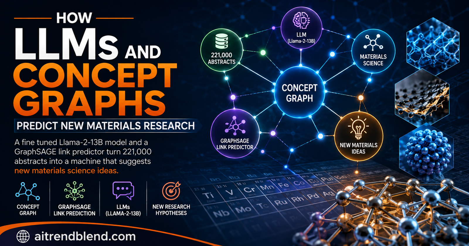
A materials scientist sits down with a fresh stack of papers and already knows the stack is a rounding error. The field now publishes more abstracts in a year than any one person could read in a decade of weekends. Buried in that flood are two ideas that have never appeared in the same sentence, and joining them would open a new line of work. Finding that pair by reading is hopeless.
A team led by Pascal Friederich at the Karlsruhe Institute of Technology decided to let a machine do the joining instead, and then asked ten working scientists whether the machine had anything useful to say.
Key points
- Roughly 221,000 materials science abstracts became a concept graph of about 137,000 nodes and 13 million edges, built by a fine tuned Llama model that extracts concepts far more cleanly than rule based keyword tools.
- The strongest predictor, a mixture of a graph neural network and MatSciBERT concept embeddings, reached a test AUC of 0.9433 for guessing which concept pairs would connect in future papers.
- Adding semantic meaning from language embeddings helped most for distant pairs, lifting recall at a previous distance of three from under 6 percent to more than 35 percent.
- Ten materials scientists reviewed personalized suggestions and rated about 26 percent of them genuinely interesting. The model own curation step nearly doubled the hit rate over a plain baseline.
- The design goal is recall over precision. The system surfaces promising ideas for a human to judge rather than trying to replace the judging.
The problem is not a shortage of ideas, it is a shortage of attention
Promising research directions often come from welding together two concepts that nobody has welded before. An experienced scientist carries a private map of their own field and can spot a few of these joins by instinct. The trouble is that the map ends at the edge of what one person has read, and the interesting joins tend to sit across that edge, in a neighbouring subfield the scientist never had time to follow.
This is the gap the Karlsruhe group set out to close. Their framing is refreshingly modest. They are not claiming a machine can understand a paper or judge whether an idea is good. They are claiming something narrower and more testable. A machine can read the whole literature at once, notice which concepts keep drifting toward each other over the years, and hand a scientist a short list of pairs worth a second look. The judging stays with the human.
That modesty matters, and it separates this work from a certain flavour of hype about machines inventing science. The authors point back to earlier efforts on machine driven ideation such as SciMuse and ResearchAgent, and to the SemNet line of work by Krenn and colleagues that first tracked the evolution of physics as a growing graph of keywords. What was missing in the graph only approaches was meaning. A node labelled tensile strength and a node labelled molecular architecture were just two dots, and the model never knew what either dot stood for.
How the literature becomes a graph
The pipeline has three stages that are worth pulling apart, because each one hides a decision that shaped the result.
Reading the abstracts
Data came from OpenAlex, the open index of scholarly work. The team queried materials science journals and conferences, cleaned the titles and abstracts, and ended up with about 221,000 articles published between 1955 and 2022. Every abstract needed its concepts pulled out, and this is where the language model earns its place.
Older systems used RAKE, a rule based keyword extractor, and RAKE has a habit of returning fragments that read like keywords but carry no real meaning, along with errors baked in by its own statistics. Instead the team fine tuned an open model, Llama-2-13B, on 100 abstracts that a human had annotated by hand. They then ran the model on 100 more abstracts, used GPT-3.5 to flag common mistakes, corrected those by hand, and folded the larger set back into training. Doing this in rounds meant the amount of manual labelling stayed small while the extraction kept improving.
The payoff is visible in the numbers. Across the corpus the model pulled out roughly 510,000 chemical formulae and 3.6 million concepts, an average of about 2.3 formulae and 16.3 concepts per abstract. After removing duplicates that condensed to around 52,000 unique formulae and 1.24 million unique concepts. The fine tuned model also learned to normalize, turning strengthening into carbon fibre reinforcement, folding plurals into singulars, and even naming concepts that never appeared word for word in the text. The whole extraction run took about 160 GPU hours.
Building the concept graph
With concepts in hand, the team built what they call a concept graph. Two concepts that appear together in the same abstract get an edge, and that edge carries a timestamp equal to the publication date. To keep the graph meaningful they only kept concepts that showed up at least three times and that consisted of at least two words, which trims the noise of one off phrases and bare single words. The result is a multigraph of about 137,000 nodes and 13 million edges.
Because every edge is dated, the graph is really a stack of graphs, one for each moment in time. A snapshot at year t keeps only the edges from papers published up to and including t. That time structure is the whole game, because predicting a new research direction means predicting which edge appears next.
Every abstract becomes a fully connected clique of its own concepts, and the dates on the edges turn the literature into a movie of how ideas connected over decades rather than a single frozen picture.
Giving the nodes meaning
Here is the move that sets the paper apart. Rather than treat each concept as an anonymous dot, the team gave every node a 768 number vector that captures what the concept means, using MatSciBERT, a version of BERT trained on materials science text. For a concept such as mechanical stress, the model tokenizes the phrase, finds every place it occurs across the abstract, embeds those positions, and averages them. When a concept does not appear verbatim, for example because the extraction normalized it, the mean is taken over all tokens in the abstract as a stand in. Average again across every abstract where the concept appears and you get one stable vector per node.
To make sure the vectors carry real meaning, the authors ran nearest neighbour queries and found that a concept sits close to its genuine cousins in the space. To picture the whole thing they projected every vector down to two dimensions with UMAP and produced what they nicely call a map of materials science, a landscape where dense yellow regions mark crowded topics and the outskirts hold the rarer ones. An interactive version lives at inspire.aimat.science if you want to wander through it.
Predicting the next edge
Link prediction sounds abstract until you frame it the way the paper does. Take two concepts that are not yet connected. Will a future paper connect them? That is a yes or no question, so the whole task collapses into binary classification over pairs of nodes.
The catch is brutal imbalance. Between 2017 and 2019 there were about 18.7 billion possible new edges, and only 1.3 million actually formed, which is around seven thousandths of one percent. Train naively on that and the model learns to say no every time and score almost perfectly. To fight this the team oversampled positives so that roughly 30 percent of each training batch was a real emerging edge. That deliberately trades precision for recall, and the authors are open about why they want that trade. Missing a good idea is worse than flagging a few bad ones, because a person is going to read the list anyway.
The equations behind the features
The baseline model, a descendant of the densely connected network from Krenn and colleagues, describes each node with only two graph properties per year. It counts how many neighbours a node has and how many two step paths pass through it, gathered across a window of years.
The concept embedding model throws those hand made counts away and feeds the raw MatSciBERT vectors instead. For a concept that appears at token positions in a set of abstracts, its node vector is a plain average.
The best model does not choose between structure and meaning. It runs a graph neural network on the topology, runs a second model on the embeddings, and blends their two output probabilities with a fixed weight.
The graph branch uses a two layer GraphSAGE encoder with neighbour sampling, which matters because the graph is large and hub heavy, and full message passing would choke on the densest nodes. A small multilayer perceptron then reads the concatenated node vectors and returns a probability. To avoid leaking the future into the past, every embedding used for a given prediction was computed only from text available up to that year.
What the numbers actually say
The team measured everything with the area under the ROC curve, which suits an imbalanced problem because it does not care about the base rate of positives. They trained on the years up to 2016, made predictions for 2017 through 2019, and tested on a held out set from 2020 to 2022 containing 2 million candidate pairs, of which only 307 turned into real edges.
| Model | Input signal | Test AUC |
|---|---|---|
| Baseline network | Graph features | 0.9109 |
| Graph neural network | Graph features | 0.9288 |
| Concept embeddings | MatSciBERT | 0.8855 |
| Network on plain BERT | BERT | 0.8547 |
| Combination of features | Graph plus MatSciBERT | 0.9147 |
| Mixture of baseline and embeddings | Graph plus MatSciBERT | 0.9372 |
| Mixture of GNN and embeddings | Graph plus MatSciBERT | 0.9433 |
Three lessons fall out of that table. First, structure and meaning are not rivals. Every hybrid beats either ingredient alone, and the top score of 0.9433 comes from mixing the graph neural network with the embeddings. Second, domain training pays. MatSciBERT at 0.8855 clears plain BERT at 0.8547, which tells you that a model tuned on materials text reads these concepts more sharply than a generic one. Third, the graph neural network at 0.9288 edges past the hand built baseline at 0.9109, so learned structure beats counted structure even before any language meaning enters.
The authors also checked their baseline against Science4Cast, a public benchmark from the Krenn group, where it scored an AUC of 0.9088 and ranked second among all reported approaches. A deep network on a large set of meaningful features can hold its own against methods built on common neighbours and node2vec style embeddings.
The distance test that reveals the real value
The headline AUC hides the most interesting finding. The team split the emerging edges by the shortest path that already existed between the two concepts, a quantity they call the previous distance. Of the 307 true new edges in the test set, 290 joined concepts that were already two hops apart and only 17 joined concepts three hops apart. Short hops dominate because the graph is so densely tangled.
Those rare three hop connections are exactly the ones a human would never guess, because the two ideas live in different corners of the field. And this is where the language embeddings prove their worth. The plain baseline caught these distant links with a recall of only 5.9 percent, essentially blind to them. The concept embedding model lifted that to 35.3 percent, a jump the authors report as statistically significant by a DeLong test. Semantic meaning, it turns out, is what lets the system reach across the graph rather than nibbling at the obvious.
The high number of false positives, especially at a previous distance of three, is not a problem in itself because those combinations may remain scientifically plausible and will subsequently be evaluated by human scientists. Hence, we prioritize recall over precision in order not to miss valuable ideas. Marwitz and colleagues, Nature Machine Intelligence, 2026
Ten scientists in a room
A high AUC on a held out set is one thing. Convincing a working scientist that a suggestion is worth their afternoon is another, and this is the part of the paper that earns real trust. The team invited thirteen materials scientists, ten agreed, and each received a personalized report. The report was built by intersecting the concepts from that scientist own recent papers with the wider graph, then ranking combinations the model thought were promising, and finally asking a language model to write a short paragraph on why each pairing might matter.
The scientists then sat for a thirty minute interview and sorted each suggestion into buckets. Already known, split into published and trivial. Nonsense. Interesting. Uncertain. Across 292 sorted suggestions, 71 were already published, 36 were trivial, 99 were nonsense, 77 were interesting, and 9 were uncertain. So about 26 percent landed as genuinely interesting to a domain expert, which is a strong hit rate for a machine reaching into a specialist field.
The curation step mattered too. When a language model was asked to pre select the interesting combinations, its precision against expert judgement was about 47 percent, meaning that of 53 pairings the model flagged, 24 also struck the scientists as interesting. Left uncurated the rate was 61 of 266, around 23 percent. Filtering with the model roughly doubled the odds that a suggestion would land.
Of nine concept pairs sitting at a previous distance of three, the hardest and least obvious cases, five were rated interesting by the experts. The connections that look absurd on a graph are often the ones worth chasing in a lab.
Some of the flagged pairings read like the start of a real proposal. Conventional ceramic with graphene oxide, aimed at composites that stay stable while conducting charge. Multiphase structure with selective laser melting, a route to printed parts with tuned phase distributions. Stress induced phase transformation with hexagonal boron nitride, borrowing a toughening trick from zirconia and asking whether boron nitride can do the same. None of these are guaranteed to work. All of them are the kind of cross topic hunch a busy researcher rarely has time to form. If you want a broader tour of how language models are moving into this field, our companion piece on multimodal LLMs for materials science covers a very different attack on the same problem, reading a crystal structure rather than the literature around it.
Where it falls short
The authors are unusually candid about the limits, and a fair reading has to sit with them.
The expert study is small. Ten interviews cannot carry statistical weight, and the participants were chosen rather than sampled at random, so some selection bias is baked in. The authors call the human findings qualitative and anecdotal, and that is the honest label. The judging task is also slippery, since scientists disagreed with themselves. A suggestion filed as nonsense in one part of an interview sometimes flipped to interesting later, once the person imagined how it might actually be built.
The precision is genuinely low, by design. Prioritizing recall means the lists are long and padded with false positives, and a user has to be willing to wade. That is fine for a brainstorming aid and would be useless as an automated filter. The distant connections, the most valuable ones, are also the sparsest, so the model has the least data exactly where it matters most. Seventeen true three hop edges is not much to learn from.
There are quieter caveats too. The concept extraction was tuned in 2023 on models that were state of the art then, and the authors note that newer models would likely sharpen the pipeline. The graph inherits whatever biases live in the literature, so a topic that was fashionable will look more connected than one that was quietly important. And a suggestion that is scientifically plausible is not the same as a suggestion that is fundable, safe, or worth the years it would take to test.
Why this line of work matters
Step back and the appeal is clear. The same recipe, extract concepts with a tuned language model, build a timestamped graph, enrich the nodes with meaning, and predict the next edge, is not tied to materials science at all. Any field with a large body of abstracts could be poured into the same machine. The authors say as much, and the door is wide open for chemistry, catalysis, battery research, or drug discovery. Readers curious about the last of those can see a related idea in our look at generative optimization of peptide antibiotics, where a model searches a space of edits rather than a graph of concepts.
The graph neural network angle also connects to a wider current in the field. Learning on graphs, rather than on grids or sequences, keeps proving useful wherever the data is really a web of relationships, from remote sensing to molecular property prediction. Our write up on manifold aware graph fusion for radar imagery shows the same GraphSAGE family at work on a completely different signal. For the broader map of how these methods fit together, see our graph neural networks pillar, which the site owner should point at the hub page once it exists.
What lingers most is the philosophy. The team could have chased a system that tries to be a scientist, and instead they built one that tries to be a good research assistant, the kind who has read everything and quietly slides a note across the desk that says these two might go together. That is a smaller claim than machine creativity, and a far more useful one.
A reference implementation
The code below is a compact, runnable version of the mixture idea. It builds the baseline graph features, stands in MatSciBERT vectors with random tensors so the demo stays light, runs a two layer GraphSAGE encoder, blends the graph branch and the embedding branch one to one, trains with oversampled positives, and scores itself with ROC AUC on dummy data. The real code and data from the authors are linked under the code.
# Predicting new research directions in materials science
# Compact reference for link prediction on a semantics aware concept graph
# Blends GraphSAGE topology with MatSciBERT style concept embeddings

import torch
import torch.nn as nn
import torch.nn.functional as F
from torch.utils.data import DataLoader, TensorDataset
from sklearn.metrics import roc_auc_score


# 1. Baseline graph features
# For each node, degree and number of two step paths, per snapshot year.
def graph_features(adj_by_year):
    feats = []
    for A in adj_by_year:
        degree = A.sum(dim=1, keepdim=True)            # node degree
        two_paths = (A @ A).sum(dim=1, keepdim=True)   # length two paths
        feats.append(torch.cat([degree, two_paths], dim=1))
    return torch.cat(feats, dim=1)


# 2. Frozen concept embeddings, a stand in for precomputed MatSciBERT vectors
class ConceptEmbedding(nn.Module):
    def __init__(self, emb_matrix):
        super().__init__()
        self.emb = nn.Embedding.from_pretrained(emb_matrix, freeze=True)

    def forward(self, node_ids):
        return self.emb(node_ids)


# 3. GraphSAGE encoder, two layers of mean aggregation
class SAGELayer(nn.Module):
    def __init__(self, in_dim, out_dim):
        super().__init__()
        self.lin_self = nn.Linear(in_dim, out_dim)
        self.lin_neigh = nn.Linear(in_dim, out_dim)

    def forward(self, x, adj_norm):
        neigh = adj_norm @ x                       # mean of neighbour features
        return F.relu(self.lin_self(x) + self.lin_neigh(neigh))


class GraphSAGE(nn.Module):
    def __init__(self, in_dim, hid_dim, out_dim):
        super().__init__()
        self.l1 = SAGELayer(in_dim, hid_dim)
        self.l2 = SAGELayer(hid_dim, out_dim)

    def forward(self, x, adj_norm):
        h = self.l1(x, adj_norm)
        return self.l2(h, adj_norm)


# 4. Edge decoder, concatenate two node vectors and score a link
class EdgeDecoder(nn.Module):
    def __init__(self, node_dim, hidden=128):
        super().__init__()
        self.net = nn.Sequential(
            nn.Linear(2 * node_dim, hidden),
            nn.ReLU(),
            nn.Dropout(0.3),
            nn.Linear(hidden, 1),
        )

    def forward(self, z_u, z_v):
        pair = torch.cat([z_u, z_v], dim=1)
        return torch.sigmoid(self.net(pair)).squeeze(-1)


# 5. Mixture of GNN and embeddings, blended one to one
class MixtureModel(nn.Module):
    def __init__(self, base_dim, emb_matrix, w_gnn=0.5):
        super().__init__()
        self.sage = GraphSAGE(base_dim, 256, 128)
        self.gnn_dec = EdgeDecoder(128)
        self.concept = ConceptEmbedding(emb_matrix)
        self.emb_dec = EdgeDecoder(emb_matrix.size(1))
        self.w_gnn = w_gnn

    def forward(self, base_x, adj_norm, u, v):
        z = self.sage(base_x, adj_norm)
        p_gnn = self.gnn_dec(z[u], z[v])
        p_emb = self.emb_dec(self.concept(u), self.concept(v))
        return self.w_gnn * p_gnn + (1.0 - self.w_gnn) * p_emb


# 6. Training loop, positives already oversampled to about 30 percent
def train(model, base_x, adj_norm, pairs, labels, epochs=5, lr=1e-3):
    opt = torch.optim.Adam(model.parameters(), lr=lr)
    loss_fn = nn.BCELoss()
    loader = DataLoader(TensorDataset(pairs, labels), batch_size=256, shuffle=True)
    for epoch in range(epochs):
        model.train()
        total = 0.0
        for pb, lb in loader:
            u, v = pb[:, 0], pb[:, 1]
            opt.zero_grad()
            pred = model(base_x, adj_norm, u, v)
            loss = loss_fn(pred, lb.float())
            loss.backward()
            opt.step()
            total += loss.item()
        print(f"epoch {epoch + 1}  loss {total / len(loader):.4f}")


# 7. Evaluation with ROC AUC
@torch.no_grad()
def evaluate(model, base_x, adj_norm, pairs, labels):
    model.eval()
    u, v = pairs[:, 0], pairs[:, 1]
    pred = model(base_x, adj_norm, u, v)
    return roc_auc_score(labels.numpy(), pred.numpy())


# 8. Runnable smoke test on dummy data
if __name__ == "__main__":
    torch.manual_seed(0)
    num_nodes, years = 200, 3

    adj_by_year = []
    for _ in range(years):
        M = (torch.rand(num_nodes, num_nodes) > 0.9).float()
        M = ((M + M.t()) > 0).float()
        M.fill_diagonal_(0)
        adj_by_year.append(M)

    base_x = graph_features(adj_by_year)             # [200, 6]

    A_last = adj_by_year[-1]
    deg = A_last.sum(dim=1, keepdim=True).clamp(min=1)
    adj_norm = A_last / deg                           # row normalized for mean aggregation

    emb_matrix = torch.randn(num_nodes, 768)         # stand in for MatSciBERT

    pos = torch.randint(0, num_nodes, (300, 2))
    neg = torch.randint(0, num_nodes, (700, 2))
    pairs = torch.cat([pos, neg], dim=0)
    labels = torch.cat([torch.ones(300), torch.zeros(700)])

    model = MixtureModel(base_x.size(1), emb_matrix)
    train(model, base_x, adj_norm, pairs, labels, epochs=3)
    auc = evaluate(model, base_x, adj_norm, pairs, labels)
    print(f"dummy AUC {auc:.4f}")
Go to the source
Read the peer reviewed paper and run the authors own code and data.
Read the paper Code on GitHubConclusion
The core achievement here is a working pipeline that reads the materials science literature end to end, turns it into a graph where the nodes actually know what they mean, and predicts which unconnected ideas will meet in a future paper. The top model, a mixture of a graph neural network and MatSciBERT embeddings, reached a test AUC of 0.9433, and it did so on a problem with a positive rate near seven thousandths of one percent, which is a genuinely hard needle in a genuinely large haystack.
The conceptual shift is the part worth remembering. For years, graph based forecasts of science treated concepts as anonymous nodes and squeezed predictions out of raw topology. This work shows that pouring semantic meaning into the nodes changes what the model can reach. The gain was small on the easy short range links and dramatic on the hard long range ones, lifting recall on distant pairs from under 6 percent to more than 35 percent. Meaning is what lets a machine jump across the field instead of shuffling along its dense interior.
The approach travels well. Nothing in the recipe is specific to metals and ceramics. Extract concepts, date the edges, enrich the nodes, predict the next link, and you have a template that any literature heavy discipline could adopt. That transferability is arguably a bigger contribution than the single materials science result, because it hands the whole method to fields that never had a SemNet of their own.
The honest remaining limits keep the work grounded. The human evaluation rested on ten interviews, the precision is low by choice, and the most valuable distant links are also the rarest and hardest to learn. A plausible suggestion is not a validated one, and the model has no idea whether an idea is safe, fundable, or already quietly failed in someone unpublished notebook. None of this sinks the result. It simply marks the line between a research assistant and a researcher.
Future directions almost write themselves. Swap in a newer extraction model, fold in the full text rather than only abstracts, add the graph neural network earlier in the study rather than late, and run the same interviews at a larger scale in a second field. If those steps hold up, the quiet note slid across the desk becomes a habit rather than a demo, and that would be a real change in how a scientist decides what to work on next.
Frequently asked questions
What does the model actually predict?
It predicts links in a concept graph. Given two materials science concepts that have never appeared together in a paper, the model estimates the probability that a future paper will use them together, which stands in for a new research direction worth exploring.
Why use a large language model to extract the concepts?
Older rule based tools such as RAKE return noisy fragments and carry statistical errors. A fine tuned Llama model reads the abstract in context, normalizes phrasing, and even names concepts that are not spelled out word for word, which produces a cleaner and more meaningful graph.
How good are the predictions?
The best mixture model reached an area under the ROC curve of 0.9433 on a held out test set from 2020 to 2022. In interviews, ten materials scientists rated about 26 percent of the personalized suggestions as genuinely interesting.
What is the point of the previous distance analysis?
It measures how far apart two concepts already sit in the graph. Distant pairs are the least obvious and most valuable suggestions, and adding semantic embeddings lifted recall on those distant pairs from 5.9 percent to 35.3 percent, which shows where meaning helps most.
Can this method work outside materials science?
Yes in principle. The pipeline of concept extraction, a timestamped graph, semantic node vectors, and link prediction does not depend on the subject. Any field with a large corpus of abstracts could apply the same approach.
Is the code available to try?
Yes. The authors released their code on Zenodo and GitHub under an open licence, and the processed graph and feature vectors are on figshare, so the results can be reproduced and extended.