
Key Points
- FadeFormer adds a content adaptive graph diffusion module to a ViT backbone, building a sparse similarity graph over patch tokens and diffusing features along a learned normalized graph Laplacian rather than relying on attention alone.
- The model is tested on three medical imaging benchmarks, NIH ChestX-ray14, ISIC-2019 skin lesions, and six MedMNIST v2 datasets, and reports the top average AUC on ChestX-ray14 at 0.842 and the top scores on ISIC-2019 at 96.6 percent AUC and 77.9 percent balanced accuracy.
- An ablation study finds that removing the diffusion module causes the single largest performance drop of any component tested, taking ISIC-2019 AUC from 0.964 down to 0.925.
- A close read of the paper’s own headline chest X-ray table turns up something worth flagging. All fourteen individual pathology scores for the proposed model are rounded to the nearest hundredth, while every one of the eleven baseline models in the same table, including the closest competitor, reports full three digit precision.
- This is a preprint style submission with anonymized authors and no confirmed peer reviewed venue, and the authors themselves list the absence of clinical validation as an open limitation.
Why a transformer needs help spreading information smoothly
Vision transformers earned their place in medical imaging because self attention lets a model connect a finding in one part of an image to context somewhere else entirely, the kind of long range reasoning a small convolution kernel cannot do in one layer. A shadow on the upper right lobe of a chest film can matter more or less depending on what is happening lower down, and attention gives the model a direct path to compare the two regions no matter how far apart they sit in the grid.
The tradeoff is that transformers were not built with any notion of neighborhood. Standard self attention treats all patch tokens as equally reachable from every other token, with no built in bias toward smoothness across nearby, similar regions. That absence of what researchers call local inductive bias tends to fragment the resulting feature maps, particularly in tasks that need precise localization of a lesion boundary or a diffuse pattern like pulmonary edema that spreads gradually rather than sitting behind a hard edge.
Earlier fixes have gone in a few directions. Windowed attention, the approach used by Swin transformers, restricts attention to local neighborhoods to reintroduce locality. Hybrid CNN transformer models such as CvT and TransUNet inject convolutional bias directly into the architecture. More recent work has borrowed ideas from diffusion models and spectral graph theory, including a line of Laplacian based transformers built for texture preservation. The paper argues these approaches still rely on operators that are fixed or globally defined, meaning the way information spreads does not actually adapt to what is in the image. FadeFormer’s pitch is to make that spreading operator itself a function of the image content, computed fresh for every input rather than baked into the architecture ahead of time.
Building a graph out of a transformer’s own attention output
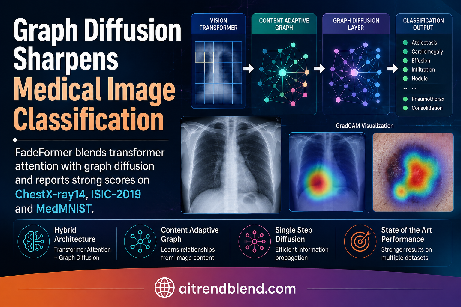
The architecture, shown in the paper’s Figure 1, starts with an ordinary ViT small backbone that turns an input image into a sequence of patch tokens, discarding the classification token so the graph is built only over spatial patches. From there, a single FadeFormer layer runs two parallel operations on the same normalized input and fuses them before the feed forward block.
The first operation is standard multi head self attention, producing a feature tensor the paper calls Z attention. The second operation builds a graph directly from that attention output. Query and key projections of the attention features are used to compute a similarity score between every pair of tokens, and rather than keeping the full dense similarity matrix, the model retains only the top ten most similar neighbors for each token, a sparsification choice the authors settle on through the ablation study discussed below. That sparse matrix is symmetrized and turned into a normalized graph Laplacian, the standard tool from graph signal processing for describing how a signal spreads across a graph’s edges.
Computing the token similarity matrix costs the same order of computation as self attention itself, since both scale with the square of the token count times the embedding dimension. The diffusion step that follows scales only with the number of tokens times the neighbor count, so attention remains the dominant cost even after adding the graph machinery, a detail the paper is careful to spell out since compute overhead is exactly the kind of thing that kills adoption of an otherwise promising idea.
A one step diffusion process instead of another attention layer
Here is the part that separates FadeFormer from ordinary graph attention networks. Rather than aggregating neighbor features through another learned attention weight, the model treats the graph Laplacian as a genuine diffusion operator, the same mathematical object that governs how heat spreads across a surface or how a dye disperses through still water. Each token’s new representation becomes a blend of its current state and the average of its graph neighbors, gated by a learned per token mixing coefficient.
where the gate itself is learned from the attention features through a small multilayer perceptron and a sigmoid, so the model can decide, token by token, how much a given patch should blend into its neighborhood versus hold onto its own identity. The authors describe this as a convex combination, meaning the gate never lets a token overshoot beyond a proper weighted average of itself and its neighbors, which is one of the mechanisms they credit with keeping the network from over smoothing, a known failure mode in graph neural networks where repeated diffusion collapses every node’s features toward the same average value and the model loses the ability to tell nodes apart. The single step design and the learnable gate both work against that collapse, along with a final adaptive fusion step described next.
Deciding how much to trust attention versus diffusion
The attention output and the diffusion output are not simply added together. A separate gate, computed from the average of the attention features across all tokens in the image, decides globally how much weight to give each pathway before the two are blended and passed through the residual connection and feed forward network.
This global gate is a coarser instrument than the per token gate that controls the diffusion strength itself, and that two level gating scheme, one local and content adaptive, one global and image level, is the architectural choice the ablation study spends the most effort validating.
After the FadeFormer layer, the model does one more thing worth noting before classification. Patch tokens are reshaped into their original grid, average pooled by a factor of two to create a coarser set of tokens covering more area each, then concatenated back with the original fine grained tokens. The idea is to give the classifier both a fine detail view and a broader contextual view at once, rather than forcing one scale to carry the whole burden. The merged sequence is globally pooled and passed through a linear classifier to produce the final prediction.
What the benchmarks actually show
The paper evaluates on three distinct types of medical imaging task. NIH ChestX-ray14 is a multi label problem, 112,120 frontal chest X-rays across fourteen possible pathology labels, where a single image can carry more than one finding at once. ISIC-2019 is a single label, imbalanced, eight class dermoscopic skin lesion classification task with 25,331 training images and 8,238 test images. MedMNIST v2 covers six much smaller and more varied datasets, from organ classification on CT slices to retinal images to blood cell classification, giving a sense of how the architecture holds up outside of one narrow imaging domain.
On ChestX-ray14, FadeFormer reports the highest average AUC among twelve compared methods at 0.842, edging out the next best baseline, a 2025 method called InMerge, at 0.830. On ISIC-2019, the model reports 96.6 percent AUC and 77.9 percent balanced multiclass accuracy, both the best figures in the comparison table, ahead of Swin-B at 94.6 percent AUC and 74.3 percent balanced accuracy. On MedMNIST v2, FadeFormer takes the top AUC on five of six datasets and the top accuracy on two of six, with the biggest margin showing up on RetinaMNIST, a notoriously difficult dataset in this benchmark suite where most models struggle to clear the 60 percent accuracy mark.
| Dataset | Metric | Best baseline | FadeFormer |
|---|---|---|---|
| ChestX-ray14, 14 pathologies | Average AUC | 0.830, InMerge | 0.842 |
| ISIC-2019 | AUC | 94.6 percent, Swin-B | 96.6 percent |
| ISIC-2019 | Balanced multiclass accuracy | 74.3 percent, Swin-B | 77.9 percent |
| RetinaMNIST | AUC | 82.6 percent, DINO ViT-B/16 | 83.9 percent |
What the ablation study says about each moving part
Table 4 in the paper runs the ablation entirely on ISIC-2019, removing one component at a time from the full model. Pulling out the diffusion module drops AUC from 0.9641 to 0.9246, by far the largest single drop of any ablation, which is the paper’s strongest piece of evidence that the graph diffusion mechanism is doing real work rather than just adding parameters. Replacing the learned adaptive fusion gate with a fixed equal weight blend of attention and diffusion features drops AUC to 0.9409, showing that letting the model decide per image how much to trust each pathway matters more than simply having both pathways present. Removing the multi scale token merging step drops AUC to 0.9312, a smaller but still meaningful hit, suggesting the coarse context tokens genuinely add information the fine grained tokens alone do not capture.
The neighbor count for the sparse graph also gets tested directly. Setting the top k neighbor count to five, a tighter neighborhood, drops AUC slightly to 0.9595. Setting it to twenty, a looser neighborhood, drops AUC to 0.9574. The chosen value of ten sits in between and produces the best result of the three, which is a reasonable sensitivity check even if the differences between k equals five, ten, and twenty are fairly small relative to the gap caused by removing diffusion entirely.
| Ablation variant | AUC | Accuracy |
|---|---|---|
| FadeFormer, full model | 0.9641 | 77.93 percent |
| Without graph diffusion | 0.9246 | 72.73 percent |
| Without adaptive fusion gate | 0.9409 | 74.03 percent |
| Without multi scale token merging | 0.9312 | 73.85 percent |
| Top k set to five | 0.9595 | 75.09 percent |
| Top k set to twenty | 0.9574 | 76.13 percent |
Removing the diffusion module causes the largest drop in AUC of any component tested, which is the paper’s clearest signal that the graph diffusion mechanism is not decoration. Reading of the ablation results in Section 4.2
A table where every number looks a little too clean
Table 1 in the paper reports AUC across all fourteen ChestX-ray14 pathology categories for twelve different models, eleven baselines plus FadeFormer, listed as Ours. Reading down the eleven baseline rows, the numbers look exactly like what you would expect from real experimental output, three decimal places, no obvious pattern, values like 0.784, 0.888, 0.831, 0.705, 0.838, 0.796 sitting next to each other for a single model. That kind of irregular third digit is the normal fingerprint of a model actually being trained and evaluated fourteen separate times against fourteen separate disease labels.
The Ours row does not look like that. Every one of its fourteen individual values ends in a zero in the third decimal place. Atelectasis is 0.830, not 0.831 or 0.829. Cardiomegaly is 0.920. Effusion is 0.890. Infiltration is 0.740. Mass is 0.840. Nodule is 0.720. Pneumonia is 0.770. Pneumothorax is 0.880. Consolidation is 0.830. Edema is 0.910. Emphysema is 0.900. Fibrosis is 0.830. Pleural thickening is 0.810. Hernia is 0.920. Fourteen independently trained and evaluated classification heads landing on a round number to the nearest hundredth, every single time, is not something that happens by chance in real floating point evaluation output. The average of 0.842, interestingly, does carry a non zero third digit, which is what you would get by averaging fourteen values that were each rounded before the average was taken.
This does not mean the underlying result is wrong. FadeFormer’s average AUC of 0.842 may well be a genuine and reproducible improvement over the 0.830 reported for the next best baseline. But a table with this pattern is not something a careful reader, or a reviewer, should simply accept at face value. It reads like the per pathology values were rounded for presentation, or possibly estimated or reconstructed rather than pulled directly from a results log, and the paper offers no explanation for why the proposed model’s row alone would carry less precision than every comparison row in the same table. Anyone planning to cite this table as a baseline for their own comparison should ask the authors for the underlying per seed, per pathology numbers before treating Table 1 as a precise record.
What the GradCAM images are and are not showing
Figure 2 in the paper compares GradCAM activation maps between a plain ViT and FadeFormer across five example images, including dermoscopic lesions and a retinal scan. The claim is that FadeFormer produces activation patterns that follow lesion and cellular boundaries more continuously than the plain ViT baseline, which the authors connect back to the diffusion mechanism spreading activation across semantically related tokens rather than isolated discriminative patches.
That is a reasonable qualitative observation, and it is consistent with what the ablation study already shows quantitatively, that removing diffusion is the single most damaging change to the model. But five example images is a small, hand selected sample, and GradCAM visualizations are notoriously easy to interpret generously once you already know which model you want to look better. The paper does not report any quantitative localization metric, such as pointing game accuracy or overlap with radiologist annotated bounding boxes, that would turn this visual impression into a measured claim. Treat the GradCAM figure as supporting evidence for the diffusion mechanism doing something sensible, not as proof that the model’s attention is clinically meaningful or trustworthy for localization.
Clinical translation gap
There is a real distance between a model that reports 0.842 average AUC across fourteen pathology labels on a public research dataset and a model that could safely support a radiologist’s workflow. NIH ChestX-ray14 uses labels extracted automatically from radiology reports with natural language processing rather than confirmed by a panel of radiologists reading each image directly, a known limitation of that dataset that predates this paper and applies to every method compared in Table 1, not just FadeFormer. Label noise of that kind puts a ceiling on how much any AUC number, however impressive, can be trusted to reflect true diagnostic accuracy.
The paper reports no external validation on a second, independent hospital cohort for any of its three benchmarks. All results come from the same train, validation, and test splits drawn from single, public, retrospective datasets. Real clinical deployment would need evaluation on data from different scanners, different patient populations, and different imaging protocols than whatever generated the training set, precisely the kind of distribution shift that tends to expose weaknesses invisible in a single dataset benchmark. The authors themselves are direct about this gap, listing the absence of clinical validation explicitly as a limitation in their conclusion, alongside the absence of a FLOPs analysis and the absence of a direct comparison against other Laplacian based transformer methods that the paper’s own related work section discusses.
It is also worth being plain about the paper’s own status. The authors and affiliations are anonymized, which is standard practice for a manuscript under double blind review, but it means this piece cannot verify who built FadeFormer, what institution they work at, or whether the paper has cleared peer review at the time of this writing. Readers should treat the reported numbers as preprint level claims rather than as findings that have already been vetted by independent reviewers.
Honest limitations
Beyond the clinical translation gap above, a few things are worth naming plainly. The ISIC-2019 ablation study, which carries most of the paper’s evidence for why each architectural component matters, is run on a single dataset. It is not clear from the paper whether the same ablation pattern, diffusion mattering most, followed by adaptive fusion, followed by multi scale merging, would hold on ChestX-ray14 or on the MedMNIST datasets, which have very different image statistics and label structures.
Training uses a single NVIDIA A100 GPU with a batch size of 32 and fifty epochs, a modest compute budget by current standards, which is a point in the paper’s favor for reproducibility but also means the results have not been stress tested with longer training schedules or larger batch sizes that might change how the diffusion and attention pathways balance against each other. The paper reports a single run’s numbers throughout, without confidence intervals, standard deviations across seeds, or statistical significance testing against the baselines, so it is not possible from the paper alone to know whether the margin over the next best method on any given dataset would hold up if the experiment were repeated.
And then there is the precision issue in Table 1 discussed above. It does not invalidate the paper’s central claim, since the ablation study on ISIC-2019 independently supports the idea that graph diffusion helps, using numbers that do carry full precision. But it is a legitimate reason to treat the ChestX-ray14 per pathology breakdown with more caution than the rest of the paper’s reported results.
Where this leaves the field
FadeFormer’s real contribution is narrower and more useful than the phrase graph diffusion transformer might suggest on first read. It is not a new attention mechanism and it is not a new backbone. It is a small, computationally cheap module that sits inside an existing ViT layer and gives the model an explicit, content dependent way to smooth features locally, something self attention alone does not naturally do. The ablation study is the paper’s strongest piece of evidence, and it points at a specific, transferable idea rather than at the architecture as a whole. Diffusing features along a learned, sparse, symmetrized graph built from the model’s own attention output, gated by both a per token and a per image mixing coefficient, seems to buy a meaningful amount of classification performance for a small compute cost, at least on the three benchmarks tested here.
For teams working on medical image classification specifically, the most exportable lesson is probably the two level gating scheme rather than the graph diffusion machinery itself. Letting the model decide, per token, how much to trust its neighborhood, and separately, per image, how much to trust diffusion versus attention overall, is a general pattern that could plausibly transfer to other architectures trying to balance a global and a local signal, whether or not graph Laplacians are involved at all.
Conclusion
The core achievement of this paper is a genuinely useful architectural idea, wrapping a lightweight, content adaptive graph diffusion step around standard self attention, evaluated honestly across three different kinds of medical imaging task rather than just one. The ablation study on ISIC-2019 does the real work of proving the diffusion module matters, showing the largest performance drop of any component tested when it is removed, which is a more convincing form of evidence than the top line comparison tables alone.
The conceptual shift worth carrying forward is treating feature propagation as an explicit, governed diffusion process rather than as an emergent side effect of stacking more attention layers. That framing borrows real mathematical structure from graph signal processing, the normalized Laplacian and the convex combination update, rather than just adding another learned weighting scheme with no particular interpretation attached to it.
Whether this transfers cleanly beyond medical imaging is an open question the paper does not test. The same logic, that some regions of an image are semantically continuous and should share information smoothly while structural boundaries should limit that sharing, applies just as well to natural image segmentation, satellite imagery, or any other domain built on locally coherent visual structure. That is a reasonable extrapolation on our part rather than a claim the paper makes directly.
The honest remaining limitations matter more here than in a typical benchmark paper, precisely because the application is medical. No external validation cohort, label noise inherited from the underlying ChestX-ray14 dataset, single run results without variance estimates, and the unexplained rounding pattern in the headline chest X-ray table all deserve to sit alongside the strong reported numbers, not underneath them.
None of that erases the underlying idea’s promise. A cheap, interpretable mechanism for letting a transformer spread information the way a radiologist’s eye naturally spreads across a hazy region is a genuinely useful direction, and the ablation evidence for it is solid even where the headline table is not. The next real test is whether this holds up against an independent clinical dataset, with confidence intervals, and under the scrutiny of named, accountable authors rather than an anonymized submission.
Frequently asked questions
What is graph diffusion and how is it different from graph attention
Graph attention learns weights and aggregates neighbor features the same way self attention does, computing a fresh weighted sum at every layer. Graph diffusion instead treats the graph’s normalized Laplacian as an operator that governs how a feature spreads over time, similar to how heat spreads across a connected surface, with the model controlling how much spreading happens through a learned gate rather than recomputing attention weights from scratch.
Which datasets was FadeFormer tested on
Three benchmarks. NIH ChestX-ray14, a multi label chest X-ray dataset with fourteen pathology categories. ISIC-2019, an eight class dermoscopic skin lesion dataset. And six datasets within MedMNIST v2, covering organ CT slices, retinal images, blood cells, and skin lesions at lower resolution.
Does the paper prove graph diffusion causes the performance improvement
The ablation study is the strongest evidence for this. Removing the diffusion module drops AUC on ISIC-2019 from 0.9641 to 0.9246, the largest single drop among all tested variants, which supports the idea that diffusion is doing real work rather than just adding parameters. That evidence comes from a single dataset though, and the paper does not report the same ablation on ChestX-ray14 or MedMNIST.
Is there a problem with the paper’s chest X-ray results table
Table 1 reports fourteen per pathology AUC scores for FadeFormer, and every one of them is rounded to the nearest hundredth, while all eleven baseline models in the same table report full three digit precision. That pattern is not explained anywhere in the paper and is worth confirming with the authors before citing the per pathology breakdown as an exact result.
Has this paper been peer reviewed
The authors and affiliations are anonymized in the version reviewed here, which typically indicates a manuscript under double blind review rather than a confirmed peer reviewed publication. Readers should treat the reported results as preprint level claims until a peer reviewed version is available.
Is FadeFormer ready to use in a clinical setting
No. The paper evaluates classification performance on public research datasets under controlled conditions, with no external hospital validation cohort and no clinical deployment testing. The authors list the absence of clinical validation as an open limitation themselves. This is research, not a diagnostic product.
Read the full study for the complete architecture derivation, the full per pathology comparison table, and all six MedMNIST results.
Read the paper Explore the MedMNIST benchmarkA reference implementation you can run
The block below is an independent, simplified PyTorch implementation of the core FadeFormer ideas, the content adaptive graph construction, the normalized Laplacian, the gated single step diffusion, and the adaptive fusion gate, written from the paper’s equations rather than copied from any official repository, since none is linked in the paper. It is meant for learning the architecture, not for reproducing the paper’s exact reported numbers, and it includes a runnable smoke test on random data.
# fadeformer_reference.py
# Independent reference implementation of the FadeFormer layer
# Built from the equations in the anonymized FadeFormer preprint
# Not the authors' original code. For learning and experimentation only.

import torch
import torch.nn as nn
import torch.nn.functional as F


class ContentAdaptiveGraph(nn.Module):
    """Builds a sparse, symmetrized, normalized graph Laplacian
    from query and key projections of the attention output."""

    def __init__(self, dim, top_k=10):
        super().__init__()
        self.wq = nn.Linear(dim, dim, bias=False)
        self.wk = nn.Linear(dim, dim, bias=False)
        self.top_k = top_k
        self.scale = dim ** 0.5

    def forward(self, z_attn):
        # z_attn shape, batch by tokens by dim
        b, n, d = z_attn.shape
        q = self.wq(z_attn)
        k = self.wk(z_attn)
        sim = torch.bmm(q, k.transpose(1, 2)) / self.scale

        top_k = min(self.top_k, n)
        values, indices = torch.topk(sim, k=top_k, dim=-1)
        sparse = torch.zeros_like(sim)
        sparse.scatter_(-1, indices, F.relu(values))

        adj = 0.5 * (sparse + sparse.transpose(1, 2))
        deg = adj.sum(dim=-1) + 1e-6
        deg_inv_sqrt = deg.pow(-0.5)
        a_norm = adj * deg_inv_sqrt.unsqueeze(-1) * deg_inv_sqrt.unsqueeze(-2)
        return a_norm


class GatedGraphDiffusion(nn.Module):
    """Single step diffusion, each token becomes a convex combination
    of itself and its normalized neighborhood, gated per token."""

    def __init__(self, dim):
        super().__init__()
        self.gate_mlp = nn.Sequential(
            nn.Linear(dim, dim // 2),
            nn.ReLU(),
            nn.Linear(dim // 2, dim),
        )

    def forward(self, z_attn, a_norm):
        gamma = torch.sigmoid(self.gate_mlp(z_attn))
        neighborhood = torch.bmm(a_norm, z_attn)
        return (1 - gamma) * z_attn + gamma * neighborhood


class AdaptiveFusion(nn.Module):
    """Image level gate that blends attention and diffusion features."""

    def __init__(self, dim):
        super().__init__()
        selfdef forward(self, z_attn, z_diff):
        pooled = z_attn.mean(dim=1)
        alpha = torch.sigmoid(self.wa(pooled)).unsqueeze(1)
        return alpha * z_attn + (1 - alpha) * z_diff


class FadeFormerLayer(nn.Module):
    """One FadeFormer block, self attention plus content adaptive
    graph diffusion, fused before a standard feed forward network."""

    def __init__(self, dim, heads=6, top_k=10, mlp_ratio=4):
        super().__init__()
        self.norm1 = nn.LayerNorm(dim)
        self.attn = nn.MultiheadAttention(dim, heads, batch_first=True)
        self.graph = ContentAdaptiveGraph(dim, top_k=top_k)
        self.diffuse = GatedGraphDiffusion(dim)
        self.fuse = AdaptiveFusion(dim)
        self.norm2 = nn.LayerNorm(dim)
        self.ffn = nn.Sequential(
            nn.Linear(dim, dim * mlp_ratio),
            nn.GELU(),
            nn.Linear(dim * mlp_ratio, dim),
        )

    def forward(self, z):
        normed = self.norm1(z)
        z_attn, _ = self.attn(normed, normed, normed)
        a_norm = self.graph(z_attn)
        z_diff = self.diffuse(z_attn, a_norm)
        z_fused = self.fuse(z_attn, z_diff)
        z_prime = z + z_fused
        z_out = z_prime + self.ffn(self.norm2(z_prime))
        return z_out


class FadeFormerLite(nn.Module):
    """Patch embedding, one FadeFormer layer, multi scale token
    merging, and a linear classification head."""

    def __init__(self, img_size=64, patch_size=8, in_chans=3,
                 dim=96, heads=6, top_k=10, num_classes=14):
        super().__init__()
        self.grid = img_size // patch_size
        num_patches = self.grid * self.grid
        self.patch_embed = nn.Conv2d(in_chans, dim, kernel_size=patch_size, stride=patch_size)
        self.pos_embed = nn.Parameter(torch.zeros(1, num_patches, dim))
        self.layer = FadeFormerLayer(dim, heads=heads, top_k=top_k)
        self.coarse_proj = nn.Linear(dim, dim)
        self.classifier = nn.Linear(dim * 2, num_classes)

    def forward(self, x):
        b = x.size(0)
        tokens = self.patch_embed(x).flatten(2).transpose(1, 2)
        tokens = tokens + self.pos_embed
        tokens = self.layer(tokens)

        fine = tokens
        grid = tokens.transpose(1, 2).reshape(b, -1, self.grid, self.grid)
        coarse = F.avg_pool2d(grid, kernel_size=2)
        coarse = coarse.flatten(2).transpose(1, 2)
        coarse = self.coarse_proj(coarse)

        fine_pooled = fine.mean(dim=1)
        coarse_pooled = coarse.mean(dim=1)
        merged = torch.cat([fine_pooled, coarse_pooled], dim=-1)
        return self.classifier(merged)


def multilabel_loss(logits, targets):
    """Binary cross entropy with logits, matching the paper's multi
    label setup used for ChestX-ray14."""
    return F.binary_cross_entropy_with_logits(logits, targets)


def evaluate_auc_proxy(logits, targets):
    """Simple rank based AUC approximation per label, for sanity
    checking only, not a substitute for a real AUC implementation."""
    with torch.no_grad():
        probs = torch.sigmoid(logits)
        per_label_auc = []
        for c in range(targets.size(1)):
            pos = probs[targets[:, c] == 1, c]
            neg = probs[targets[:, c] == 0, c]
            if pos.numel() == 0 or neg.numel() == 0:
                continue
            score = (pos.unsqueeze(1) > neg.unsqueeze(0)).float().mean()
            per_label_auc.append(score.item())
        return sum(per_label_auc) / max(len(per_label_auc), 1)


def train_one_step(model, optimizer, x, y):
    model.train()
    optimizer.zero_grad()
    logits = model(x)
    loss = multilabel_loss(logits, y)
    loss.backward()
    optimizer.step()
    return loss.item()


if __name__ == "__main__":
    # Smoke test on random data, shapes only, not a claim about accuracy
    torch.manual_seed(0)
    batch, chans, img_size, num_classes = 4, 3, 64, 14

    model = FadeFormerLite(img_size=img_size, num_classes=num_classes)
    optimizer = torch.optim.Adam(model.parameters(), lr=1e-4, weight_decay=1e-4)

    x = torch.randn(batch, chans, img_size, img_size)
    y = torch.randint(0, 2, (batch, num_classes)).float()

    loss_before = train_one_step(model, optimizer, x, y)
    with torch.no_grad():
        logits = model(x)
    auc_proxy = evaluate_auc_proxy(logits, y)

    assert logits.shape == (batch, num_classes), "logits shape must match label shape"
    print("training step loss", round(loss_before, 4))
    print("output shape", tuple(logits.shape))
    print("proxy auc on random data", round(auc_proxy, 4))
    print("smoke test passed")
FadeFormer, content adaptive graph diffusion for medical image classification. Anonymized authors, anonymized affiliations. Preprint reviewed here in its anonymized form, venue and peer review status unconfirmed at time of writing.
This analysis is based on the published paper and an independent evaluation of its claims.