
Key Points
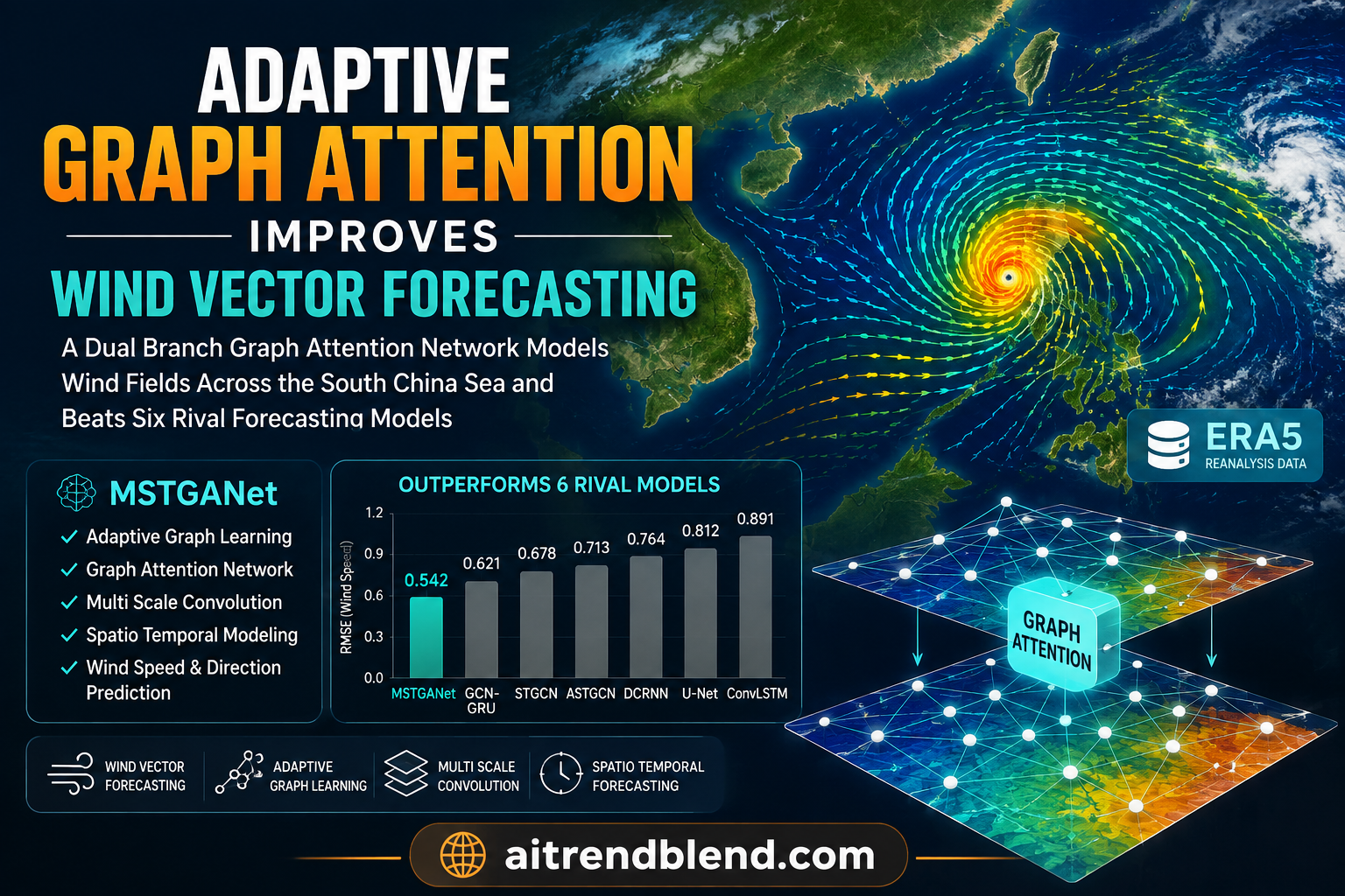
- MSTGANet pairs a four branch 3D convolutional encoder with two separately learned adjacency matrices and a dual attention module to forecast the U and V wind components 24 hours ahead over the South China Sea.
- The model trains on nine years of ERA5 reanalysis data at 100 meter hub height and is tested against six established forecasting architectures including U-Net, ViT, ConvLSTM, and a rival spatio temporal graph transformer called STGTN.
- An ablation test surfaces a real warning for anyone stacking graph convolution and attention layers. Wiring them together directly, without an intermediate transform, produced the single worst result among seven tested variants, trailing even a plain CNN.
- A careful read of the paper’s own wind direction accuracy table shows the eight way and sixteen way angle tolerance columns are identical for every model at every forecast horizon, a pattern that should not occur if the two tolerances were computed independently.
- Transfer tests on eastern China and northwestern China, regions with very different wind regimes than the South China Sea, hold up well at short horizons, which says something about how much of what the model learns is genuinely physical rather than tied to one coastline.
What a wind vector actually asks a model to predict
Wind speed forecasting has a long history built on physical simulation, statistical time series methods, and more recently deep networks. Global wind capacity keeps climbing, and China alone added 80 gigawatts in 2024, which the paper notes was roughly seventy percent of everything the world added that year. That scale of build out raises the stakes on getting the forecast right, because a grid absorbing that much variable generation needs to know not just how hard the wind will blow but which way it will come from.
Most of the forecasting literature treats wind as a single number at a single point. That framing misses something obvious once you say it out loud. Wind is a three dimensional field that moves across a region over time, shaped by monsoon circulation in the South China Sea and occasionally torn apart by a typhoon. A forecast built from one weather station tells you almost nothing about the farm two ridgelines over. So researchers have been shifting toward grid based and multi site prediction, treating each grid cell as a node in a graph and letting the network learn how those nodes relate to each other.
The authors frame their task cleanly. Given the U and V wind components (the east west and north south pieces of the vector) over the past 24 hours across a grid, predict the same two components for the next 24 hours. U and V together carry both speed and direction, since speed is just the vector magnitude and direction falls out of the angle between them. That is a more demanding target than speed alone, and it is the reason the paper introduces its own accuracy metric for direction rather than borrowing one wholesale from meteorology.
Where this sits among graph based forecasting methods
Graph neural networks became a natural fit for grid wind data because a wind field is not really a flat image. Distance matters, but so do relationships a simple grid of pixels cannot represent, like the way a coastal breeze correlates with a station forty kilometers inland more than with a station five kilometers away across open water. Earlier work built adjacency matrices from fixed rules such as geographic distance. More recent systems, including the DAGLN framework from Ren and colleagues and the adaptive graph learning convolutional network from Liu and colleagues, let the network learn the graph structure itself rather than hand coding it.
MSTGANet borrows that instinct but splits it in two. The authors argue, reasonably, that a single learned adjacency matrix is being asked to represent two very different physical processes at once. Local turbulence and terrain effects create short range correlations that decay quickly with distance. Monsoon and typhoon circulation create long range correlations that do not care about distance at all. Forcing one matrix to capture both means it probably does neither particularly well, a point the authors credit to the dual branch design in a related paper called STCADFN.
| Item | Detail |
|---|---|
| Training region | South China Sea, 110E to 119E, 17N to 26N |
| Data source | ERA5 reanalysis from ECMWF, U and V wind at 100 meter height |
| Time span | Hourly data 2015 through 2024 |
| Split | 2015 to 2022 training, 2023 validation, 2024 test |
| Task | Predict the next 24 hours from the previous 24 hours |
| Transfer regions | Eastern China (114E to 123E, 29N to 38N) and northwestern China (95E to 104E, 32N to 41N) |
Four branches looking at the same sky in different ways
The first module in the pipeline is a multi scale 3D convolutional encoder, and the design choice here is worth sitting with. Instead of one convolution trying to capture every spatial scale, the authors run four parallel branches over the same input tensor, each with a different kernel footprint. A one by three by three kernel handles fine local variation, the kind of turbulent eddy or terrain driven gradient that only shows up over a small patch. A three by five by five kernel targets mesoscale structure such as sea land breeze cycles. A five by seven by seven kernel is aimed at synoptic scale patterns, meaning monsoon fronts and the wide spiral of a typhoon. A fourth branch with a seven by one by one kernel looks only along the time axis, tracking how a single location evolves without mixing in neighboring cells.
Each branch produces its own feature map through convolution, batch normalization, and a ReLU activation. The four outputs are concatenated along the channel dimension and passed through a one by one by one convolution that compresses the combined features back down, with dropout applied for regularization. The resulting tensor keeps the original spatial and temporal resolution, which matters because every later module, including the graph learning stage, depends on having one feature vector per grid node per timestep to work with.
Learning two different graphs instead of forcing one to do both jobs
This is the part of the paper that carries the most conceptual weight. Rather than hand building an adjacency matrix from geographic distance, the model learns two embedding matrices per node, one local and one global, and derives an adjacency matrix from each through a dot product and a ReLU nonlinearity.
The local branch and its grid mask
The local branch computes a similarity matrix between node embeddings, then multiplies it element by element with a grid mask built from Manhattan distance. Any pair of nodes within a distance of two, roughly a three by three neighborhood, gets a weight that falls off as 1 over (1 plus distance). Anything farther gets zeroed out entirely. That is a hard physical prior baked directly into the architecture. It tells the model, from the first training step, to trust nearby correlations before it trusts distant ones, which the authors say speeds convergence and stabilizes training.
The global branch and its constant bias
The global branch skips the distance mask entirely and adds a flat bias of 0.1 to every entry after the ReLU step. That small addition keeps weak long range connections alive in the graph rather than letting them collapse to exactly zero, which matters if the model is going to have any chance of picking up on a typhoon track that connects two grid cells hundreds of kilometers apart. Both matrices then go through symmetric Laplacian normalization before being handed to the graph convolution stage, which keeps the propagation numerically stable regardless of how many neighbors a given node happens to have.
Fusing local and global signal through parallel graph convolution
Once the two adjacency matrices exist, the dual branch graph convolutional network applies each one separately to the encoded features, then passes the aggregated result through its own two layer multilayer perceptron. That keeps the local and global pathways from contaminating each other during the aggregation step itself. Only after both branches have produced their own representation does the model concatenate them and pass the combined vector through a linear fusion layer that projects back down to a working dimension.
This two stage separation before fusion is a deliberate structural choice, and the ablation results later in the paper make a strong case for why it matters. Bolting components together without an intermediate transformation step, it turns out, can actively hurt performance rather than help it.
Where the model chooses to look, in space and in time
After fusion, a spatial attention module assigns each node an importance score between zero and one through a fully connected layer and a sigmoid, then multiplies that score back onto the node features. The authors report, and this is one of the more interpretable findings in the paper, that the learned weights consistently land on coastlines, complex terrain, and the eyewall region of typhoons once one is present in the input window. That is a sensible place for a model to concentrate attention, since those are exactly the zones where wind speed gradients are sharpest and where a small error in position translates into a large error in predicted intensity.
A multi head temporal attention module follows, computing query, key, and value projections across the time dimension and letting the model weigh which historical hours matter most for a given forecast step. This is standard scaled dot product attention split across multiple heads, the same mechanism that made the Transformer architecture dominant in sequence modeling generally, applied here to the temporal axis of a spatially weighted feature sequence rather than to raw tokens.
A direct decoder and a search driven optimizer
Rather than predicting one hour ahead and feeding that prediction back in as input for the next hour, which is how recurrent forecasting systems typically work, MSTGANet outputs all 24 future hours in a single pass through a multilayer perceptron decoder that reshapes its output back into gridded U and V fields. Direct multi step prediction like this avoids the error accumulation that recursive decoding is prone to, at the cost of losing whatever benefit autoregressive feedback might otherwise provide during longer horizons.
Hyperparameters, including dropout rate, learning rate, encoder channel counts, graph convolution hidden dimension, attention head count, and weight decay, are tuned with an algorithm the authors call AGDO, short for Adam gradient descent optimization, which blends Adam style adaptive moment estimates with a heuristic global search. The tuned values landed at a dropout rate near 0.14, a learning rate of 0.0004, 199 and 228 channels in the two encoder stages, a graph convolution hidden dimension of 231, and 7 attention heads.
| Parameter | Tuned value |
|---|---|
| Dropout rate | 0.136 |
| Learning rate | 0.0004 |
| Encoder channels, stage 1 | 199 |
| Encoder channels, stage 2 | 228 |
| GCN hidden dimension | 231 |
| Attention heads | 7 |
| Weight decay | 1.05e minus 6 |
What seven ablation variants reveal, including one that fails badly
The authors test seven configurations, labeled L1 through L7, moving from a plain CNN baseline up to the full model. L1 is CNN alone, L2 adds attention to the CNN, L3 is GCN alone, L4 is GCN with attention bolted directly on, L5 is CNN plus GCN without deep integration, L6 is the full CNN GCN attention stack, and L7 is the complete AGDO tuned MSTGANet.
Two results stand out. First, L3 (GCN alone) clearly beats L1 (CNN alone) across almost every horizon and metric, which supports the paper’s central claim that graph convolution suits the non-Euclidean structure of wind data better than a convolution built for flat images. Second, and far more interesting, L4 is the worst performer of all seven variants, worse even than the plain CNN it was supposed to improve on. For the 24 hour U component prediction, L4 posts an R squared of 0.48, compared to 0.59 for the plain CNN L1 and 0.74 for the full model L7.
The authors offer a physically grounded explanation rather than shrugging this off as noise. A graph convolution acts as a low pass filter, smoothing node features by averaging over neighbors and reducing the variance that distinguishes one node from the next. An attention mechanism does close to the opposite job, computing pairwise similarity and sharpening the contrast between features so it can decide what to weight heavily. Chain those two operations directly, with no transformation layer in between to reconcile them, and you get exactly what you would expect from combining a blur filter with a sharpen filter in the wrong order. Gradients become unstable, the discriminative signal attention needs gets smoothed away before it can be used, and the smoothed representation the GCN worked to build gets torn apart by the sharpening step right after. Model L5, which just stacks CNN and GCN features by concatenation, does better than L1 and L2 but still falls short of L3 alone, suggesting that shallow stacking without real architectural integration carries its own penalty, just a smaller one than L4’s.
| Variant | Components | 24h R squared, U | 24h R squared, V |
|---|---|---|---|
| L1 | CNN only | 0.59 | 0.62 |
| L2 | CNN plus attention | 0.62 | 0.66 |
| L3 | GCN only | 0.62 | 0.69 |
| L4 | GCN with attention bolted on | 0.48 | 0.51 |
| L5 | CNN plus GCN, shallow stack | 0.62 | 0.67 |
| L6 | Full stack, no AGDO tuning | 0.69 | 0.74 |
| L7 | Full MSTGANet with AGDO tuning | 0.74 | 0.78 |
The number in Table 16 that does not add up
Reading the paper’s ablation tables closely turns up something the authors do not comment on anywhere in the text. Table 16 reports wind direction accuracy for the seven model variants at three angle tolerances, four bins, eight bins, and sixteen bins, across five forecast horizons. Narrowing the tolerance from eight bins to sixteen bins should almost always lower the reported accuracy, since a sixteen way split demands the predicted angle land within a much tighter window than an eight way split does. Yet in Table 16, the eight bin and sixteen bin columns are identical, digit for digit, for every one of the seven models at every one of the five horizons. ConvLSTM reports 84.63 percent at both eight bins and sixteen bins for the one hour forecast. MSTGANet reports 94.26 percent at both eight bins and sixteen bins for the same horizon. That pattern holds all the way through the twenty four hour column too.
Compare that with Table 11, the earlier ablation table covering the L1 through L7 variants rather than the six baseline comparisons. There, the eight bin and sixteen bin values are genuinely different from each other and decline in the direction you would expect as the tolerance tightens. L1 at one hour reports 82.58 percent at eight bins and 78.82 percent at sixteen bins, a believable four point gap. Whatever produced Table 16 clearly did not repeat that same computation, or copied one column into the other during table assembly. It does not undermine the paper’s broader argument, since the R squared, RMSE, MAE, and ACC comparisons in Tables 12 through 15 do not depend on this particular table, but it is exactly the kind of detail a careful reader should flag rather than skim past, and it is a reminder that even a well built experimental section can carry a transcription error that slips through review.
A graph convolution smooths, an attention layer sharpens, and wiring them together with nothing in between is closer to running a blur filter and a sharpen filter back to back than it is to building a richer model. Reading of the L4 ablation result in Section 4.4
How MSTGANet compares against six established forecasting models
The headline comparison pits MSTGANet against U-Net, ViT, ConvLSTM, GCN-GRU, Windformer, and STGTN, all trained and tested on the identical South China Sea dataset. MSTGANet wins on every metric at every horizon, but the size of the margin tells its own story. At one hour ahead, several rivals are already close. ViT reaches an R squared of 0.97 on the U component at one hour, matching MSTGANet’s own 0.97. The gap opens up as the horizon stretches. By 24 hours, ViT’s U component R squared has fallen to 0.69, a 27 percent relative decline in U-Net’s case specifically, while MSTGANet only drops to 0.74.
The paper attributes ViT’s steeper decline to the absence of any explicit spatial topology modeling, since a plain vision transformer treats the grid as a sequence of patches rather than as a graph with physically meaningful neighbor relationships. Windformer, a Transformer built for wind forecasting specifically, holds up better over long horizons but still trails MSTGANet across the board, which the authors chalk up to the same missing ingredient, no explicit graph structure. STGTN is the closest architectural cousin here, since it also combines graph structure with attention, and it does outperform the purely recurrent models. But its 24 hour U component R squared of 0.66 sits well below MSTGANet’s 0.74, and the paper argues this comes down to STGTN using a single static graph rather than the dual adaptive local and global structure MSTGANet learns.
To back the comparison statistically, the authors run a Diebold Mariano test between MSTGANet and each baseline at four representative horizons. Every comparison clears the 1.96 significance threshold by a wide margin. The gap against STGTN is the largest, with DM statistics ranging from about 16 to 27 across horizons, while the gap against ViT is the smallest, sitting between roughly 6.5 and 7.8. That pattern is consistent with what the raw R squared numbers already suggested, ViT is the closest competitor and STGTN, despite sharing the graph plus attention idea, ends up furthest behind.
| Model | 24h R squared, U | 24h RMSE, U (m/s) | DM statistic vs MSTGANet, 24h |
|---|---|---|---|
| ConvLSTM | 0.63 | 2.69 | 12.39 |
| GCN-GRU | 0.66 | 2.57 | 12.34 |
| STGTN | 0.66 | 2.60 | 16.44 |
| U-Net | 0.70 | 2.45 | 8.97 |
| ViT | 0.69 | 2.46 | 6.50 |
| Windformer | 0.73 | 2.30 | 5.00 |
| MSTGANet | 0.74 | 2.28 | n/a |
Typhoons, calm days, and what a heatmap can and cannot show you
Numbers in a table are one thing. The paper also plots gridded predictions against ground truth for two contrasting scenarios, a typical low wind day and Typhoon Yagi, a genuinely severe storm. On the calm day, ConvLSTM and GCN-GRU produce overly smooth fields that miss local variation entirely, STGTN misjudges the spatial extent of the one region with elevated wind speed, and Windformer gets close but still blurs the boundary of that zone. MSTGANet is the only model whose predicted field visually tracks both the location and the gradual evolution of the higher speed patch across the full 24 hour window.
The typhoon case is more demanding, and the model differences become more visible. ConvLSTM and GCN-GRU fail to locate the storm’s high speed core at all. STGTN renders only a diffuse blob where the core should be. ViT underestimates the core’s intensity. U-Net gets the intensity roughly right but misjudges its spatial extent. MSTGANet is reported to track the core’s position, intensity, and structural evolution across the full forecast window, including at 24 hours, where the paper says the residual structure of the predicted high speed zone still lines up with the observed field. That is the scenario that matters most operationally, since a grid operator cares far more about getting the typhoon forecast right than about shaving a fraction of a degree off a calm day prediction.
Training on one coastline, testing on two very different ones
Transfer results are where the paper makes its strongest claim about practical usefulness. A model trained entirely on South China Sea data is applied without retraining to eastern China, a region shaped by land sea interaction with wind speeds mostly between 3 and 9 meters per second, and to northwestern China, an inland region with a more uniform 3 to 6 meter per second regime dominated by northerly winds. At the one hour horizon, R squared reaches 0.90 for eastern China and 0.91 for northwestern China, both close to what the model achieves on its home region. Wind direction accuracy at the loosest tolerance also holds up, landing at 94.6 percent and 94.9 percent respectively, nearly matching the South China Sea numbers.
Accuracy does fall off faster over the transfer regions as the horizon extends. By 6 hours, R squared for the U component drops to 0.66 in eastern China and 0.57 in northwestern China, a steeper decline than the model shows on its training region at the same horizon. That gap is worth sitting with rather than glossing over, since it suggests the model’s short term skill generalizes well but its longer range forecasting ability is more tied to patterns specific to the South China Sea climate it was trained on. Still, achieving useful one hour and three hour accuracy in a region with a completely different wind regime, without a single gradient update on that region’s data, is a genuinely useful property for anyone trying to stand up wind forecasting for a new site without collecting years of local training data first.
Honest limits worth naming
A few things temper how far these results should be trusted. The maximum training epoch count is fixed at 10 for every model in the comparison, which is a thin budget for architectures this large and raises the question of whether some baselines, particularly Windformer and STGTN, were left short of their own convergence point. The evaluation is entirely reanalysis against reanalysis, meaning ERA5 predictions are compared against other ERA5 values rather than against independent buoy or station observations, so any systematic bias already present in ERA5 itself would not show up as an error here. The test period covers a single year, 2024, which limits how much can be said about performance across a wider range of storm seasons. And as already discussed, the paper’s own wind direction accuracy table for the baseline comparison shows an internal inconsistency between its eight bin and sixteen bin columns that the authors do not address, which is reason enough to treat that particular set of numbers cautiously until clarified. None of this erases the core result, that the dual graph design and the AGDO tuned architecture outperform six established alternatives on the metrics that were computed correctly, but a careful reader should hold the direction accuracy claims in Table 16 a little more loosely than the speed metrics in Tables 12 through 15.
Where this leaves the field
MSTGANet’s core contribution is not any single novel layer. Multi scale convolution, adaptive graph learning, and spatio temporal attention have all appeared separately in prior work. What the paper demonstrates is that combining them carefully, with explicit local and global graph separation and a properly staged fusion step rather than a naive concatenation, produces a meaningfully better result than any of its parts alone, and that the order and manner of combination matters enormously, as the L4 ablation failure makes clear. The transfer experiments push the argument further, suggesting the learned representations capture something closer to general atmospheric physics than to South China Sea specific quirks, at least over short horizons.
For teams building similar systems, the most exportable lesson may be the negative one. If you are stacking graph convolution and attention, do not assume the combination automatically helps. The smoothing behavior of a GCN and the sharpening behavior of an attention layer can actively fight each other without an intermediate transformation to reconcile them, and this paper offers a rare documented case where that failure mode produced a worse model than either component running alone.
Conclusion
The core achievement here is straightforward to state even if the architecture behind it is not. By learning two separate graphs instead of one, and by staging graph convolution and attention through proper fusion rather than direct connection, MSTGANet delivers measurably better wind vector forecasts than six established alternatives across every tested horizon, and it does so while also producing a usable wind direction forecast, a target most of the comparison models were never built to handle well in the first place.
The conceptual shift worth carrying forward is the idea that a single learned adjacency matrix is often being asked to do two jobs it cannot do equally well at once. Local turbulence and long range circulation are physically different processes with different spatial signatures, and splitting the graph learning task in two, with a physically grounded mask constraining the local branch and an unconstrained but bias stabilized global branch, gave the model room to specialize rather than compromise.
The transfer results point toward something broader than wind forecasting specifically. Any spatio temporal field problem where local and long range dependencies both matter, air quality modeling, ocean current prediction, even certain epidemiological spread models, could plausibly borrow the dual graph idea rather than the wind specific details of this particular architecture. That is speculative on our part rather than something the paper tests directly, but the underlying logic does not depend on wind physics in particular.
The honest remaining limitations are real. Ten epochs of training per model is a short budget for a fair comparison. Testing against reanalysis data rather than ground station observations leaves open whether ERA5’s own biases are quietly baked into every number reported. And the Table 16 inconsistency this piece flags deserves a correction or an explanation from the authors, even if it does not touch the paper’s central speed forecasting claims.
None of that undercuts the practical case for taking this architecture seriously. A wind forecasting model that holds up under typhoon conditions, transfers to unfamiliar climates without retraining, and gives operators a usable direction forecast alongside the speed number is a genuine step forward for a field that has mostly optimized for speed alone. The next test will be whether it holds up against real station data and a longer training run, not just against reanalysis and ten epochs.
Frequently asked questions
What makes MSTGANet different from earlier graph based wind forecasting models
Most earlier graph neural network approaches to wind forecasting learn a single adjacency matrix meant to capture all spatial relationships at once. MSTGANet learns two separate matrices instead, one constrained by a local distance mask to capture short range turbulence and terrain effects, and one left unconstrained with a small bias term to capture long range circulation patterns such as monsoon flow or typhoon tracks.
Does MSTGANet predict wind direction as well as wind speed
Yes. Because the model works directly with the U and V wind components rather than a single speed value, direction falls out naturally from the predicted vector. The authors introduce a metric called ANG to score direction accuracy at several angle tolerances, and MSTGANet outperforms all six baseline models on this metric as well as on the standard speed metrics.
What is the ablation finding about combining graph convolution with attention
When the authors connected a graph convolution layer directly into an attention layer with no transformation step between them, the resulting model performed worse than a plain convolutional network, the worst result among all seven tested variants. The explanation offered is that graph convolution smooths node features while attention sharpens them, and chaining the two without reconciliation destabilizes training.
How well does the model generalize to regions it was not trained on
A version trained only on South China Sea data was tested without any retraining on eastern China and northwestern China, two regions with different wind regimes. Short horizon accuracy held up well, close to the model’s performance on its home region, though the gap widened noticeably by the six hour mark, especially in northwestern China.
Is there a problem with any of the tables in the paper
Table 16, which reports wind direction accuracy for the baseline model comparison, shows identical values in its eight bin and sixteen bin tolerance columns for every model and every forecast horizon. Since a tighter sixteen bin tolerance should almost always report lower accuracy than an eight bin tolerance, this looks like a data or transcription error rather than a genuine result, and it is worth treating those two columns cautiously until the authors clarify.
Where can I get the code and data used in the paper
The authors published their implementation on GitHub, linked in the CTA section below, and the ERA5 reanalysis data used for training is publicly available through the Copernicus Climate Data Store operated by ECMWF.
Read the full study for the complete architecture details, all seven ablation tables, and the wind rose comparisons across three regions.
Read the paper on ScienceDirect View the code on GitHubA reference implementation you can run
The block below is an independent, simplified PyTorch implementation of the core MSTGANet ideas, the multi scale encoder, the dual adaptive graph learning module, the dual branch graph convolution with fusion, and the spatial plus temporal attention stack, written from the paper’s equations rather than copied from the authors’ repository. It is meant for learning the architecture, not for reproducing the paper’s exact reported numbers, and it includes a runnable smoke test on random data so you can confirm the shapes line up before pointing it at real ERA5 tensors.
# mstganet_reference.py
# Independent reference implementation of the MSTGANet architecture
# Built from the equations in Jian, Mo, Li and Huang, Energy and AI, 2026
# Not the authors' original code. For learning and experimentation only.

import torch
import torch.nn as nn
import torch.nn.functional as F


class MultiScaleEncoder(nn.Module):
    """Four parallel 3D convolutional branches over the same input tensor."""

    def __init__(self, in_channels, branch_channels, dropout=0.14):
        super().__init__()
        self.branch_local = self._make_branch(in_channels, branch_channels, (1, 3, 3))
        self.branch_meso = self._make_branch(in_channels, branch_channels, (3, 5, 5))
        self.branch_synoptic = self._make_branch(in_channels, branch_channels, (5, 7, 7))
        self.branch_temporal = self._make_branch(in_channels, branch_channels, (7, 1, 1))
        self.fuse = nn.Conv3d(branch_channels * 4, branch_channels * 2, kernel_size=1)
        self.dropout = nn.Dropout3d(dropout)

    def _make_branch(self, in_channels, out_channels, kernel_size):
        pad = tuple(k // 2 for k in kernel_size)
        return nn.Sequential(
            nn.Conv3d(in_channels, out_channels, kernel_size, padding=pad),
            nn.BatchNorm3d(out_channels),
            nn.ReLU(inplace=True),
        )

    def forward(self, x):
        # x shape, batch by channels by time by height by width
        f1 = self.branch_local(x)
        f2 = self.branch_meso(x)
        f3 = self.branch_synoptic(x)
        f4 = self.branch_temporal(x)
        fused = torch.cat([f1, f2, f3, f4], dim=1)
        out = F.relu(self.fuse(fused))
        return self.dropout(out)


class DualAdaptiveGraphLearning(nn.Module):
    """Learns a local, distance masked adjacency matrix and a global,
    bias stabilized adjacency matrix from separate node embeddings."""

    def __init__(self, num_nodes, embed_dim, height, width, local_radius=2):
        super().__init__()
        self.num_nodes = num_nodes
        self.local_embed = nn.Parameter(torch.randn(num_nodes, embed_dim) * 0.01)
        self.global_embed = nn.Parameter(torch.randn(num_nodes, embed_dim) * 0.01)
        self.register_buffer("grid_mask", self._build_grid_mask(height, width, local_radius))

    def _build_grid_mask(self, height, width, radius):
        coords = torch.stack(torch.meshgrid(
            torch.arange(height), torch.arange(width), indexing="ij"
        ), dim=-1).reshape(-1, 2).float()
        dist = torch.cdist(coords, coords, p=1)
        mask = torch.where(dist <= radius, 1.0 / (1.0 + dist), torch.zeros_like(dist))
        return mask

    def _normalize(self, adj):
        adj = adj + torch.eye(adj.size(0), device=adj.device)
        deg = adj.sum(dim=1)
        deg_inv_sqrt = torch.pow(deg, -0.5)
        deg_inv_sqrt[torch.isinf(deg_inv_sqrt)] = 0.0
        d_mat = torch.diag(deg_inv_sqrt)
        return d_mat @ adj @ d_mat

    def forward(self):
        a_local = F.relu(self.local_embed @ self.local_embed.t()) * self.grid_mask
        a_global = F.relu(self.global_embed @ self.global_embed.t()) + 0.1
        return self._normalize(a_local), self._normalize(a_global)


class DualBranchGraphConv(nn.Module):
    """Applies each adjacency matrix through its own two layer MLP,
    then fuses local and global representations with a linear layer."""

    def __init__(self, in_dim, hidden_dim, out_dim):
        super().__init__()
        self.local_mlp = nn.Sequential(nn.Linear(in_dim, hidden_dim), nn.ReLU(), nn.Linear(hidden_dim, out_dim))
        self.global_mlp = nn.Sequential(nn.Linear(in_dim, hidden_dim), nn.ReLU(), nn.Linear(hidden_dim, out_dim))
        self.fusion = nn.Linear(out_dim * 2, out_dim)

    def forward(self, x, a_local, a_global):
        # x shape, batch by nodes by features
        z_local = torch.einsum("ij,bjf->bif", a_local, x)
        z_global = torch.einsum("ij,bjf->bif", a_global, x)
        h_local = self.local_mlp(z_local)
        h_global = self.global_mlp(z_global)
        fused = torch.cat([h_local, h_global], dim=-1)
        return self.fusion(fused)


class SpatioTemporalAttention(nn.Module):
    """Node level spatial gating followed by multi head temporal attention."""

    def __init__(self, dim, heads=7):
        super().__init__()
        self.spatial_gate = nn.Linear(dim, 1)
        self.temporal_attn = nn.MultiheadAttention(dim, heads, batch_first=True)
        self.out_proj = nn.Linear(dim, dim)

    def forward(self, x):
        # x shape, batch by time by nodes by features
        b, t, n, f = x.shape
        alpha = torch.sigmoid(self.spatial_gate(x))
        x = x * alpha
        x = x.permute(0, 2, 1, 3).reshape(b * n, t, f)
        attn_out, _ = self.temporal_attn(x, x, x)
        attn_out = self.out_proj(attn_out)
        return attn_out.reshape(b, n, t, f).permute(0, 2, 1, 3)


class MSTGANetLite(nn.Module):
    """End to end reference model. Predicts future U and V wind fields
    from a historical window of gridded wind data."""

    def __init__(self, height, width, in_channels=2, branch_channels=16,
                 embed_dim=32, gcn_hidden=64, feat_dim=32, heads=4,
                 horizon=24):
        super().__init__()
        self.height, self.width = height, width
        num_nodes = height * width
        encoder_out = branch_channels * 2

        self.encoder = MultiScaleEncoder(in_channels, branch_channels)
        self.graph_learner = DualAdaptiveGraphLearning(num_nodes, embed_dim, height, width)
        self.graph_conv = DualBranchGraphConv(encoder_out, gcn_hidden, feat_dim)
        self.attention = SpatioTemporalAttention(feat_dim, heads=heads)
        self.decoder = nn.Sequential(
            nn.Linear(feat_dim, feat_dim * 2),
            nn.ReLU(),
            nn.Linear(feat_dim * 2, in_channels),
        )
        self.horizon = horizon

    def forward(self, x):
        # x shape, batch by channels by time by height by width
        b, c, t, h, w = x.shape
        enc = self.encoder(x)
        enc = enc.permute(0, 2, 3, 4, 1).reshape(b, t, h * w, -1)

        a_local, a_global = self.graph_learner()

        step_features = []
        for step in range(t):
            step_features.append(self.graph_conv(enc[:, step], a_local, a_global))
        seq = torch.stack(step_features, dim=1)

        attended = self.attention(seq)
        last_state = attended[:, -1]
        pooled = attended.mean(dim=1) + last_state

        preds = []
        for _ in range(self.horizon):
            preds.append(self.decoder(pooled))
        preds = torch.stack(preds, dim=1)
        preds = preds.reshape(b, self.horizon, self.height, self.width, -1)
        return preds.permute(0, 4, 1, 2, 3)


def mstganet_loss(pred, target):
    """Mean squared error over U and V components, matching the
    regression objective implied by the paper's evaluation metrics."""
    return F.mse_loss(pred, target)


def evaluate(pred, target):
    """Computes R squared, RMSE, and MAE the way Section 4.2 defines them,
    without the latitude weighting term for simplicity."""
    with torch.no_grad():
        mse = F.mse_loss(pred, target).item()
        rmse = mse ** 0.5
        mae = F.l1_loss(pred, target).item()
        target_mean = target.mean()
        ss_res = ((target - pred) ** 2).sum()
        ss_tot = ((target - target_mean) ** 2).sum()
        r2 = (1 - ss_res / ss_tot).item()
    return {"rmse": rmse, "mae": mae, "r2": r2}


def train_one_epoch(model, optimizer, x, y):
    model.train()
    optimizer.zero_grad()
    pred = model(x)
    loss = mstganet_loss(pred, y)
    loss.backward()
    optimizer.step()
    return loss.item()


if __name__ == "__main__":
    # Smoke test on random data, shapes only, not a claim about accuracy
    torch.manual_seed(0)
    batch, channels, history, height, width, horizon = 2, 2, 24, 8, 8, 24

    model = MSTGANetLite(height=height, width=width, in_channels=channels, horizon=horizon)
    optimizer = torch.optim.Adam(model.parameters(), lr=4e-4, weight_decay=1.05e-6)

    x = torch.randn(batch, channels, history, height, width)
    y = torch.randn(batch, channels, horizon, height, width)

    loss_before = train_one_epoch(model, optimizer, x, y)
    with torch.no_grad():
        pred = model(x)
    metrics = evaluate(pred, y)

    assert pred.shape == y.shape, "prediction shape must match target shape"
    print("training step loss", round(loss_before, 4))
    print("output shape", tuple(pred.shape))
    print("sanity metrics", {k: round(v, 4) for k, v in metrics.items()})
    print("smoke test passed")
Jian X, Mo X, Li H, Huang G. A novel multi scale spatio temporal graph attention network for wind vector forecasting. Energy and AI, Volume 25, 2026, article 100832. https://doi.org/10.1016/j.egyai.2026.100832
This analysis is based on the published paper and an independent evaluation of its claims.