
Key points
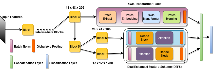
- DEF-SwinE2NET starts from EfficientNetV2S and adds exactly two things, a Swin Transformer block in the fourth stage and a Dual Enhanced Features Scheme in the last two stages, combining dilated dense convolutions with spatial and channel attention.
- Across three public MRI datasets covering glioma, meningioma, pituitary tumor and healthy scans, the full model reached accuracies of 99.08 percent, 99.43 percent and 99.35 percent, each ahead of the plain backbone and of adding either module alone.
- A four way ablation table isolates exactly how much each addition contributes, and the two modules do not duplicate each other, both improve results, and the combination beats either one used in isolation on every dataset.
- Data augmentation mattered most on the smallest of the three datasets, where accuracy fell from roughly 99 percent to under 97 percent when augmentation was switched off.
- The authors are candid about the tradeoffs, the added modules increase memory use and inference time, make the model harder to interpret and debug, and have only been validated on brain MRI so far, not on other imaging types or tumor tasks.
Why brain tumor classification resists easy wins
Brain tumors do not follow a template. The same diagnosis, glioma for instance, can show up as wildly different shapes, sizes and locations from one patient’s scan to the next, while different tumor types can sometimes look deceptively similar to each other on a single slice. That combination, high variation within a class and low separation between classes, is exactly the condition that trips up classifiers built around fixed, local convolutional filters, which is the starting point the authors use to justify reaching for both a wider receptive field and an attention mechanism rather than relying on convolution alone.
The clinical stakes explain why this matters beyond a benchmark leaderboard. Getting the tumor type right shapes the treatment path, surgery, radiation, chemotherapy, or some combination, and the paper opens by noting that brain tumors can arise from cancer spreading from elsewhere in the body, from genetic conditions, or from radiation exposure, producing symptoms from persistent headaches and seizures to personality changes that meaningfully affect a patient’s daily life. A faster, more reliable read of an MRI scan is not a purely academic goal here.
What the existing literature was still missing
The authors’ review of prior work is unusually specific about the gaps rather than settling for a generic call for more research. Comparative studies, they note, often test a narrow range of architectures rather than exploring hybrid combinations broadly. Most work relies on a single imaging dataset, which limits how much confidence anyone can have in a model’s diagnostic reliability across different scanner types and patient populations. Real time performance and computational efficiency are frequently left out of the evaluation entirely, even though a model too slow or too heavy for clinical hardware is not clinically useful no matter how accurate it is on a benchmark. And explainability, the ability to show a clinician which part of an image drove a prediction, is often treated as an afterthought rather than a design requirement.
Ensemble approaches, which combine several full models to improve accuracy, run into their own problem the authors point out directly, several ensemble members built from similar CNN architectures end up gathering the same kind of information, which limits how much a fresh member actually adds. Hybrid CNN and transformer combinations, meanwhile, tend to demand heavy computational resources. DEF-SwinE2NET is built specifically to sidestep both of those failure modes, adding just enough transformer and attention capacity to close the gap without ballooning cost.
Inside DEF-SwinE2NET, two additions to one efficient backbone
The foundation is EfficientNetV2S, chosen for a documented balance of accuracy and efficiency against alternatives like ResNet, Xception, DenseNet and the original EfficientNetV1. Everything else in this paper is about exactly where and how to graft new capability onto that foundation, rather than replacing it.
A Swin Transformer block in the fourth stage
Ordinary convolutional layers see a fixed, local neighborhood of pixels no matter how deep the network goes, which limits how well they can relate a tumor’s boundary on one side of an image to context on the far side. The Swin Transformer block, inserted specifically into the fourth block of the backbone, processes the image as a set of non overlapping patches and applies self attention within shifting windows, alternating between four sub window positions the authors label upper left, upper right, lower left and lower right, so that information can flow across window boundaries over successive layers rather than staying locked inside a single fixed window. This gives the network a genuine path to long range dependencies, patterns and relationships that span a wide area of the image, which the authors argue is exactly what distinguishing between tumor types with wildly different sizes and locations requires.
The Dual Enhanced Features Scheme in the last two stages
The second addition, applied only to the final two stages of the backbone, combines two complementary ideas the authors label a dense block with dilation and a dual attention mechanism, and the order in which they are applied is deliberately reversed between the two stages, dilation first then attention in the second to last block, attention first then dilation in the last block.
The dilated dense block widens each convolutional layer’s effective field of view without adding proportionally more parameters, by spacing out the pixels a filter samples using a dilation factor. Layers are connected densely, meaning each new layer sees the output of every previous layer in the block, which the authors describe as encouraging feature reuse and helping combat the vanishing gradient problem that can make deep networks harder to train.
That is the spatial attention half of the dual attention mechanism, where a block’s feature map \(B\) is compressed with global average pooling, passed through a dense layer with a sigmoid activation to produce spatial weights \(S_A\), then used to rescale the original feature map into \(B_A\). A parallel channel attention branch performs a similar operation but focuses on which feature channels matter most rather than which spatial locations do, and the two attention outputs are combined by element wise multiplication into a single attention weighted feature map. The practical effect is a feature map that has been told twice, once about where to look and once about what to look for, before it moves on to classification.
The preprocessing pipeline before any model sees the images
A meaningful share of this paper’s improvement comes from cleaning up the images themselves before they ever reach the network, and the authors treat that preprocessing chain as seriously as the architecture. A median filter runs first, replacing each pixel with the median value of its neighborhood to strip out noise while preserving real edges. Contrast Limited Adaptive Histogram Equalization, or CLAHE, comes next, redistributing pixel intensities within local tiles of the image to bring out subtle contrast in the tumor region while capping how aggressively any single tile can be stretched, which prevents the noise amplification that plain histogram equalization can cause. A Laplacian edge enhancement step follows, sharpening the boundaries and transitions that matter most for distinguishing a tumor’s edge from surrounding tissue. Finally, a cropping step removes the irrelevant black background common in MRI scans by finding the boundary of actual image content and discarding everything outside it, which both reduces computational load and eliminates a source of noise the model would otherwise have to learn to ignore.
Three datasets, two class structures
The evaluation draws on three public benchmark collections rather than one, which directly answers the single dataset gap the authors identified in prior work. Two Kaggle hosted datasets contribute a four class structure, glioma tumor, meningioma tumor, pituitary tumor and a healthy no tumor class, with the first containing 3,264 images and the second 7,023 images, both built from T1 weighted MRI scans. A third dataset sourced from Figshare contributes 3,064 images across three classes, dropping the healthy scan category and keeping only the three tumor types.
What the numbers show
| Dataset | Accuracy | Sensitivity | F1 score | Overall ROC-AUC |
|---|---|---|---|---|
| Kaggle Dataset 1, 4 classes, 3264 images | 99.08% | 99.19% | 99.08% | 99.98% |
| Kaggle Dataset 2, 4 classes, 7023 images | 99.43% | 99.39% | 99.41% | 99.92% |
| Figshare Dataset 3, 3 classes, 3064 images | 99.35% | 99.30% | 99.30% | 99.96% |
The confusion matrices behind these numbers are worth a closer look than the headline percentages alone. On the smallest dataset, the model missed only three cases total out of the validation set, and every one of them was a glioma case mistaken for something else. On the larger four class dataset, it missed four cases, one glioma and three meningioma, suggesting the meningioma class became slightly harder to separate as the dataset grew, a genuine tradeoff rather than a uniform improvement across every category. On the three class dataset, the two misclassifications split evenly between glioma and meningioma, which the authors read as a more balanced error pattern than either of the other two datasets showed.
Our proposed model provides better performance on the glioma class for dataset2 but decreases the performance on the meningioma class against dataset1. Abbas Malik, Saeed, Shehzad and Iqbal, Biomedical Signal Processing and Control, 2025
What the ablation study reveals about which addition earns its place
The most useful table in this paper for anyone deciding whether a similar dual addition is worth the engineering cost isolates each module’s individual contribution across all three datasets.
| Configuration | Dataset 1 accuracy | Dataset 2 accuracy | Dataset 3 accuracy |
|---|---|---|---|
| Original EfficientNetV2S alone | 96.02% | 96.73% | 97.72% |
| Plus Swin Transformer block only | 98.47% | 98.86% | 98.70% |
| Plus Dual Enhanced Features Scheme only | 98.78% | 99.29% | 99.02% |
| Full DEF-SwinE2NET, both additions | 99.08% | 99.43% | 99.35% |
Two things stand out here. First, the Dual Enhanced Features Scheme on its own consistently outperformed the Swin Transformer block on its own, across all three datasets, suggesting the dense dilated attention combination is doing more of the individual heavy lifting than the transformer addition is. Second, and just as important, combining both additions still beat either one alone on every single dataset, by margins ranging from 0.14 percentage points on the largest dataset to 0.33 percentage points on the three class dataset. Those combined gains are modest in absolute terms once each module has already done most of the work individually, but they are consistent rather than a coin flip, which supports the paper’s claim that the two mechanisms are complementary rather than redundant.
Why augmentation mattered most where the data was thinnest
The authors also tested the full model with and without the data augmentation step, rotating, flipping, zooming and adjusting brightness on training images to artificially expand the effective dataset size. The gap this opened up tracked dataset size closely. On the smallest dataset, accuracy fell from roughly 99 percent with augmentation to about 96.6 percent without it, a drop of more than two percentage points. On the two larger datasets the gap was smaller, around one and a half points on the four class Kaggle set and about one and a half points on the three class Figshare set. The pattern is exactly what a reasonable prior would predict, a model has less room to overfit when it already has thousands of real images to learn from, and augmentation earns its keep most where the underlying dataset is smallest, which is worth remembering for any brain tumor project working with a dataset closer to a few hundred than a few thousand images.
What the Grad-CAM heatmaps added
To check whether the model’s attention was actually landing on the tumor rather than on irrelevant background, the authors generated Grad-CAM heatmaps for the plain backbone and for each intermediate variant. The plain EfficientNetV2S model’s attention tended to spread diffusely across large portions of the scan, including areas with no tumor present. The full DEF-SwinE2NET model’s heatmaps concentrated much more tightly on the actual tumor region, a visual result consistent with the accuracy gains and a useful sanity check that the model is not simply getting the right answer for the wrong reasons.
How this compares against thirteen prior published methods
The authors assembled a comparison table spanning thirteen previously published brain tumor classification approaches, including transfer learning methods built on DenseNet201 and Xception, ensemble models combining CNNs with support vector machines, a spinal convolutional attention network combining CNN and transformer ideas, and a DCT-CNN-ResNet50 hybrid using discrete cosine transform based image fusion. Reported accuracies in that comparison range from roughly 93 percent up to 98.72 percent, with DEF-SwinE2NET’s 99.43 percent and 99.35 percent scores sitting above all of them. It is worth treating this kind of table with some caution, since each comparison method was evaluated on its own original dataset and setup rather than reproduced fresh under identical conditions here, but the consistent gap across such a wide range of prior approaches, spanning plain CNNs, hybrid SVM combinations and transformer hybrids alike, is a reasonably strong signal on its own.
A second comparison table looking specifically at training hyperparameters adds a useful efficiency angle to the accuracy story. Where most prior studies trained for 80, 100 or even 300 epochs using Adam or SGD optimizers with ReLU activations, DEF-SwinE2NET reached its results in just 25 epochs using the Adamax optimizer and the Swish activation function. Fewer training epochs is not automatically a virtue on its own, but paired with a leading accuracy result, it suggests the architecture and optimizer choice are converging efficiently rather than simply brute forcing performance through longer training.
The clinical translation gap
It is worth being direct about the distance between a 99 percent benchmark score and a validated clinical tool. All three datasets used here are public, retrospective collections assembled for machine learning research, sourced from Kaggle and Figshare rather than directly from hospital systems with documented clinical provenance, patient demographics or scanner variety. The paper does not report cross dataset generalization, meaning a model trained on one of these three collections was not tested against images from a different one to see whether performance holds up on data assembled by a different team with different acquisition protocols.
Inference speed and interpretability, the two practical requirements the authors themselves flagged as under addressed gaps in prior literature, remain open questions for their own model too. The discussion section acknowledges directly that real world application requires reducing inference time for real time use and improving interpretability to build clinical trust, describing this as future work rather than a solved problem.
Honest limitations
The authors lay out their own limitations in a dedicated section rather than leaving them implicit, and the list is specific rather than boilerplate. The Dual Enhanced Features Scheme, despite a minimal parameter overhead by design, can still increase memory consumption and inference time, particularly for larger scale datasets or higher resolution images than the ones tested here. The complex interactions between the dense dilated block, the dual attention mechanism and the Swin Transformer block, stacked together, make the resulting model harder to interpret and debug than a simpler architecture would be, a direct tension with the explainability goal the paper set out to address in the first place. Performance has so far been validated only on brain MRI specifically, and the authors state plainly that generalizability to other medical imaging modalities or to different tumor classification tasks entirely remains to be thoroughly tested rather than assumed.
The dataset limitation deserves its own emphasis too. Three datasets is a genuine improvement over the single dataset norm the authors criticized in prior work, but all three are still relatively small and specific by the standards of large scale medical imaging research, and the authors acknowledge directly that the limited size and diversity of the data may lead to overfitting, with generalizability to broader, more varied clinical populations still an open question.
Conclusion
The most transferable lesson in this paper is architectural discipline rather than raw scale. Rather than assembling an ensemble of many large models or building an entirely new transformer from the ground up, the authors identified two specific, well motivated gaps in a strong existing backbone, limited receptive field and weak attention to spatially relevant regions, and added the smallest components that could plausibly close each gap. The ablation table’s finding that both additions help, and that neither alone matches the combination, is exactly the kind of evidence that justifies the added complexity rather than assuming it.
The preprocessing pipeline deserves equal credit alongside the architecture. Four distinct preprocessing steps, noise reduction, contrast enhancement, edge sharpening and background cropping, were applied before the network ever saw an image, and the augmentation ablation makes clear that at least one of these interventions, data augmentation specifically, carried a measurably larger share of the improvement on the smallest of the three datasets. A reader focused only on the architecture diagram would miss a meaningful part of where this paper’s accuracy actually comes from.
What keeps the result credible rather than overstated is the authors’ own candor about where it falls short. Three public, retrospective, English language literature style benchmark datasets are not the same as prospective validation across hospital systems, scanner manufacturers and patient populations, and the authors say directly that the model’s generalizability to other imaging modalities or tumor tasks remains untested. That is exactly the right note to end a benchmark paper on, a clear result within a clearly bounded scope rather than a claim that outruns the evidence.
The tension between accuracy and interpretability that the authors flag in their own limitations section is likely to be the more interesting story going forward. Stacking dilated convolutions, dual attention and a transformer block together produced the best numbers in this study, but the same stacking is also what the authors admit makes the model harder to interpret and debug, precisely the property their introduction identified as underserved in prior brain tumor classification research. Closing that gap without giving back the accuracy gain is a harder problem than adding one more module, and it is the problem this line of research still has to solve.
Read against the broader push toward AI assisted radiology, this paper is best understood as a careful, well ablated proof that targeted architectural additions can meaningfully move a strong baseline forward on a hard, high variability classification problem. The next test that matters is whether DEF-SwinE2NET, or an architecture built on the same principle, holds up on brain MRI collected fresh from a hospital this team has never worked with, using a scanner these three datasets never included.
A working PyTorch implementation
The block below is a runnable, simplified implementation of the two core additions described in the paper, a dense block with dilated convolutions and a dual spatial plus channel attention mechanism, wired around a small convolutional backbone with a categorical cross entropy training loop, an Adamax style optimizer, and an evaluation function for accuracy, precision, sensitivity, specificity and F1 score. It is written to make the mechanics concrete rather than to reproduce the paper’s exact EfficientNetV2S and Swin Transformer backbone or its clinical datasets.
# def_swine2net_reference.py
# A compact, runnable reference implementation of the Dual Enhanced Features Scheme
# (dense block with dilation plus dual attention) from Abbas Malik, Saeed, Shehzad
# and Iqbal, Biomedical Signal Processing and Control 2025.
# This is an educational reference, not a reproduction of the paper's exact backbone.

import torch
import torch.nn as nn
import torch.nn.functional as F


class SpatialAttention(nn.Module):
    """Follows Equations 3 and 4 of the paper, global average pooling into a
    sigmoid gated per channel spatial weight."""

    def __init__(self, channels):
        super().__init__()
        self.pool = nn.AdaptiveAvgPool2d(1)
        self.fc = nn.Linear(channels, channels)

    def forward(self, x):
        b, c, _, _ = x.shape
        pooled = self.pool(x).view(b, c)
        weights = torch.sigmoid(self.fc(pooled)).view(b, c, 1, 1)
        return x * weights


class ChannelAttention(nn.Module):
    """Follows Equations 5 and 6 of the paper, two stacked sigmoid gated dense layers."""

    def __init__(self, channels):
        super().__init__()
        self.fc1 = nn.Linear(channels, channels)
        self.fc2 = nn.Linear(channels, channels)

    def forward(self, x):
        b, c, h, w = x.shape
        pooled = x.mean(dim=(2, 3))
        intermediate = torch.sigmoid(self.fc1(pooled))
        refined = torch.sigmoid(self.fc2(intermediate)).view(b, c, 1, 1)
        return x * refined


class DualAttention(nn.Module):
    """Combines spatial and channel attention following Equation 7 of the paper."""

    def __init__(self, channels):
        super().__init__()
        self.spatial = SpatialAttention(channels)
        self.channel = ChannelAttention(channels)

    def forward(self, x):
        spatial_weighted = self.spatial(x)
        channel_weighted = self.channel(x)
        return spatial_weighted * channel_weighted


class DenseDilatedBlock(nn.Module):
    """
    A dense connectivity block using dilated convolutions with a dilation rate
    of 2, following the description in Section 3.1.3 of the paper. Each layer
    sees the concatenated output of every previous layer in the block.
    """

    def __init__(self, channels, num_layers=3, growth=16, dilation=2):
        super().__init__()
        self.layers = nn.ModuleList()
        in_ch = channels
        for _ in range(num_layers):
            self.layers.append(
                nn.Sequential(
                    nn.Conv2d(in_ch, growth, kernel_size=3, padding=dilation, dilation=dilation),
                    nn.BatchNorm2d(growth),
                    nn.SiLU(),  # SiLU is the Swish activation used throughout the paper
                )
            )
            in_ch += growth
        self.project = nn.Conv2d(in_ch, channels, kernel_size=1)

    def forward(self, x):
        features = [x]
        for layer in self.layers:
            concatenated = torch.cat(features, dim=1)
            out = layer(concatenated)
            features.append(out)
        dense_out = torch.cat(features, dim=1)
        projected = self.project(dense_out)
        return projected + x


class DualEnhancedFeaturesScheme(nn.Module):
    """
    Combines the dense dilated block with dual attention, with the order
    reversed between two stages as described in Section 3.1.5 of the paper.
    """

    def __init__(self, channels, dilation_first=True):
        super().__init__()
        self.dense_block = DenseDilatedBlock(channels)
        self.attention = DualAttention(channels)
        self.dilation_first = dilation_first
        self.norm = nn.BatchNorm2d(channels)

    def forward(self, x):
        x = self.norm(x)
        if self.dilation_first:
            x = self.dense_block(x)
            x = self.attention(x)
        else:
            x = self.attention(x)
            x = self.dense_block(x)
        return x


class DEFClassifierLite(nn.Module):
    """A small convolutional backbone with DEF modules in its last two stages."""

    def __init__(self, in_channels=3, base_channels=32, num_classes=4):
        super().__init__()
        self.stem = nn.Sequential(
            nn.Conv2d(in_channels, base_channels, kernel_size=3, padding=1),
            nn.BatchNorm2d(base_channels),
            nn.SiLU(),
            nn.MaxPool2d(2),
        )
        self.stage1 = nn.Sequential(
            nn.Conv2d(base_channels, base_channels * 2, kernel_size=3, padding=1),
            nn.BatchNorm2d(base_channels * 2),
            nn.SiLU(),
            nn.MaxPool2d(2),
        )
        self.def_second_last = DualEnhancedFeaturesScheme(base_channels * 2, dilation_first=True)
        self.stage2 = nn.Sequential(
            nn.Conv2d(base_channels * 2, base_channels * 4, kernel_size=3, padding=1),
            nn.BatchNorm2d(base_channels * 4),
            nn.SiLU(),
            nn.MaxPool2d(2),
        )
        self.def_last = DualEnhancedFeaturesScheme(base_channels * 4, dilation_first=False)
        self.pool = nn.AdaptiveAvgPool2d(1)
        self.head = nn.Linear(base_channels * 4, num_classes)

    def forward(self, x):
        x = self.stem(x)
        x = self.stage1(x)
        x = self.def_second_last(x)
        x = self.stage2(x)
        x = self.def_last(x)
        pooled = self.pool(x).flatten(1)
        return self.head(pooled)


def classification_loss(logits, labels):
    # Matches the categorical cross entropy loss described in Section 4.3 of the paper.
    return F.cross_entropy(logits, labels)


@torch.no_grad()
def evaluate(model, images, labels, num_classes):
    model.eval()
    logits = model(images)
    preds = logits.argmax(dim=1)

    correct = (preds == labels).float()
    accuracy = correct.mean().item()

    # One vs rest precision, sensitivity and specificity, averaged across classes,
    # matching the confusion matrix based metrics in Equations 29 to 33 of the paper.
    precisions, sensitivities, specificities = [], [], []
    for cls in range(num_classes):
        tp = ((preds == cls) & (labels == cls)).sum().item()
        fp = ((preds == cls) & (labels != cls)).sum().item()
        fn = ((preds != cls) & (labels == cls)).sum().item()
        tn = ((preds != cls) & (labels != cls)).sum().item()

        precision = tp / (tp + fp) if (tp + fp) > 0 else 0.0
        sensitivity = tp / (tp + fn) if (tp + fn) > 0 else 0.0
        specificity = tn / (tn + fp) if (tn + fp) > 0 else 0.0

        precisions.append(precision)
        sensitivities.append(sensitivity)
        specificities.append(specificity)

    mean_precision = sum(precisions) / num_classes
    mean_sensitivity = sum(sensitivities) / num_classes
    mean_specificity = sum(specificities) / num_classes
    f1 = (
        2 * mean_precision * mean_sensitivity / (mean_precision + mean_sensitivity)
        if (mean_precision + mean_sensitivity) > 0
        else 0.0
    )

    return {
        "accuracy": accuracy,
        "precision": mean_precision,
        "sensitivity": mean_sensitivity,
        "specificity": mean_specificity,
        "f1": f1,
    }


def train_one_step(model, optimizer, images, labels):
    model.train()
    optimizer.zero_grad()
    logits = model(images)
    loss = classification_loss(logits, labels)
    loss.backward()
    optimizer.step()
    return loss.item()


def smoke_test():
    """Runs one training step and one evaluation step on random dummy data."""
    device = torch.device("cuda" if torch.cuda.is_available() else "cpu")
    torch.manual_seed(0)

    batch_size, channels, height, width, num_classes = 8, 3, 64, 64, 4
    images = torch.rand(batch_size, channels, height, width, device=device)
    labels = torch.randint(0, num_classes, (batch_size,), device=device)

    model = DEFClassifierLite(in_channels=channels, base_channels=16, num_classes=num_classes).to(device)
    # Adamax is the optimizer used throughout the paper, matching Equations 25 to 28.
    optimizer = torch.optim.Adamax(model.parameters(), lr=1e-3)

    loss_value = train_one_step(model, optimizer, images, labels)
    metrics = evaluate(model, images, labels, num_classes)

    print(f"Smoke test training loss {loss_value:.4f}")
    print(f"Smoke test metrics {metrics}")
    assert torch.isfinite(torch.tensor(loss_value))
    print("Smoke test passed")


if __name__ == "__main__":
    smoke_test()
Frequently asked questions
What does DEF-SwinE2NET stand for and what does it do
DEF-SwinE2NET combines a Dual Enhanced Features scheme with a Swin Transformer block, built on an EfficientNetV2S backbone, to classify brain MRI scans into tumor categories such as glioma, meningioma, pituitary tumor, or healthy tissue.
Can this model diagnose a brain tumor on its own
No. It is a research classification model evaluated on public retrospective benchmark datasets, not a validated diagnostic device. Any clinical use would require prospective validation, regulatory clearance and oversight by qualified radiologists and oncologists.
Which of the two added modules contributed more
The Dual Enhanced Features Scheme on its own outperformed the Swin Transformer block on its own across all three datasets, but combining both consistently beat either one alone, showing the two additions are complementary rather than redundant.
What datasets was the model tested on
Three public benchmarks, two four class Kaggle datasets with 3,264 and 7,023 T1 weighted MRI images covering glioma, meningioma, pituitary tumor and healthy scans, and a three class Figshare dataset with 3,064 images covering the three tumor types without a healthy class.
How much did data augmentation actually help
It helped most on the smallest dataset, where accuracy dropped from about 99 percent with augmentation to roughly 96.6 percent without it. The gap was smaller on the two larger datasets, consistent with augmentation mattering more when there is less real training data to begin with.
What limitations do the authors themselves point out
They note the added modules increase memory use and inference time, make the model harder to interpret and debug, have only been validated on brain MRI so far, and were tested on datasets whose limited size and diversity may lead to overfitting on broader clinical populations.
Read the full paper for the complete equations, all thirteen comparison methods and the Grad-CAM figures.
Read the paper on Biomedical Signal Processing and ControlRelated reading
Academic citation. Abbas Malik, M.G., Saeed, A., Shehzad, K. and Iqbal, M. DEF-SwinE2NET, Dual enhanced features guided with multi-model fusion for brain tumor classification using preprocessing optimization. Biomedical Signal Processing and Control, 100, 107079, 2025. https://doi.org/10.1016/j.bspc.2024.107079
This analysis is based on the published paper and an independent evaluation of its claims.
Pingback: Revolutionizing Cardiac Care with the CACTUS Framework