
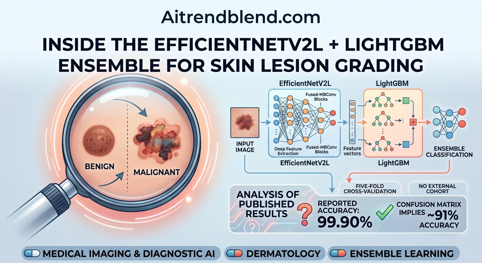
A dermatologist looking at a mole under a dermoscope has maybe ninety seconds before the next patient walks in. Fair skin, a family history, a spot that changed shape last spring. The decision to biopsy or reassure rests on pattern recognition built over years, and it still gets things wrong often enough that automated support tools keep getting proposed as a second pair of eyes. A team from Bangladesh University of Business and Technology, IISER Bhopal, NIT Jamshedpur, Amrita Vishwa Vidyapeetham, and BMS College of Engineering built one such tool, pairing a large convolutional network called EfficientNetV2L with a gradient boosting classifier called LightGBM, and published it in Results in Engineering in January 2025. The headline numbers are startling. A test accuracy of 99.90 percent in the best cross validation fold. Read past the abstract and the paper’s own figures tell a more complicated story.
Key points
- The model feeds EfficientNetV2L features into LightGBM and blends both predictions with a tunable weight, trained on 3297 dermoscopy images split into benign and malignant classes.
- Reported metrics include a training accuracy of 99.57 percent, a validation accuracy of 99.93 percent, and a five fold cross validation test accuracy of 99.90 percent in the strongest fold.
- The paper’s own confusion matrix in Figure 9 sums to an accuracy near 91 percent on the held out test set, a large gap from the headline numbers reported in the text and in Table 7.
- The per class counts inside that confusion matrix also do not match the benign and malignant test set sizes given earlier in Table 2, which is worth flagging before anyone treats this model as production ready.
- The dataset comes from a single public Kaggle source built from ISIC archive images, with no outside hospital cohort used to confirm the results hold up on lesions the model has never seen anything like.
- The architecture and the loss weighting are genuinely well documented, which makes this a useful paper to study even where the results section needs a second look.
Why another skin cancer classifier
Skin cancer sits sixth among the cancers rising fastest worldwide, and melanoma, its most lethal form, causes roughly fifty five thousand deaths a year even though it accounts for a small fraction of total cancer diagnoses. The five year survival rate for early stage melanoma runs near 98 percent, but that number collapses to somewhere between 20 and 50 percent once the disease reaches an advanced stage. The entire argument for automated screening rests on that gap. Catch it early and the outlook is good. Catch it late and it usually is not.
The conventional path to a diagnosis runs through a visual exam and, if something looks suspicious, a biopsy. Both steps depend on a clinician’s judgment and both take time a patient with a fast growing lesion may not have. The paper’s authors frame their contribution as a way to compress that timeline, not by replacing dermatologists but by giving them a fast, automatic first pass that flags a lesion as more likely benign or malignant based on the same kind of image a dermoscope produces.
Earlier attempts at this task go back further than most readers might expect. Table 1 of the paper itself lists more than a dozen prior efforts, and the pattern across them is consistent. Small datasets, a few hundred to a few thousand images, paired with convolutional networks or classic feature based methods like the ABCD rule for asymmetry, border, color, and diameter. Accuracy figures in that prior work cluster in the 77 to 98 percent range depending on the dataset and the number of classes involved, and the authors repeatedly cite overfitting and dataset uncertainty as the recurring failure mode. That framing sets up the current paper’s central claim, that a bigger and more carefully augmented dataset paired with a stronger architecture closes those gaps.
What the model actually does
The pipeline has two stages that run in sequence rather than in parallel. First, EfficientNetV2L acts as a feature extractor. Images are resized to 224 by 224 pixels for input preparation and then processed through the network at an internal working resolution of 256 by 256, After training, the paper pulls features out of the penultimate layer rather than the final classification layer. Second, those extracted deep features get combined with the raw feature representation and fed into LightGBM, a gradient boosting framework that builds an ensemble of decision trees using histogram based splitting and gradient based one side sampling to keep training fast on large feature sets.
EfficientNetV2L itself is built from two kinds of building blocks. Fused MBConv layers, which collapse the usual expansion convolution and depthwise convolution into a single regular convolution, and standard MBConv layers with squeeze and excitation attention. The paper explains that Fused MBConv trades a larger number of parameters and floating point operations for faster training in the early stages of the network, while ordinary MBConv layers stay cheaper per layer but rely on depthwise convolutions that underuse modern accelerators. Table 3 in the source paper lays out the full stack, starting with a plain 3 by 3 convolution, running through four Fused MBConv stages and three MBConv stages with channel counts climbing from 32 up to 640, and ending in a fully connected layer with 1280 channels feeding the classifier head.
Choosing how much of the network should use each block type is not something the authors hand tuned. EfficientNetV2’s original design used a neural architecture search to find that mix, and this paper adopts the resulting configuration rather than searching from scratch. The scaling across depth, width, and input resolution follows the compound scaling approach from the original EfficientNet family, where a single coefficient adjusts all three dimensions together instead of tuning them independently.
Where LightGBM comes in
Once EfficientNetV2L has produced a feature vector for every training image, LightGBM takes over. It builds decision trees iteratively, each new tree trained to correct the errors of the ensemble built so far, which is the standard gradient boosting decision tree recipe. What LightGBM adds on top of a plain gradient boosting decision tree is a histogram based approach to finding split points, which buckets continuous feature values instead of sorting every value individually, plus gradient based one side sampling, which keeps the training examples with the largest gradients and randomly samples the rest, and exclusive feature bundling, which merges features that rarely take nonzero values at the same time. Together these tricks are why LightGBM tends to train faster than older boosting libraries on wide feature sets like the ones a convolutional network produces.
The two models do not simply hand off to each other. Their final predictions get combined with a weighted average, written in the paper as a weight parameter tuned on a validation set to balance the EfficientNetV2L output against the LightGBM output. That weight is chosen to maximize a metric like accuracy or F1 score rather than fixed in advance, which is a reasonable design choice, though the paper never actually reports what value the tuned weight settled on.
Worth remembering
This is a feature extraction and ensemble architecture, not a segmentation model on its own. The lesion masks shown later in the paper come from a separate step the authors describe only briefly, and the classification accuracy claims and the segmentation quality claims should be judged independently of each other.
The math behind the training
The classification loss for a single branch of the network is a standard cross entropy over the class probabilities produced by a softmax layer.
Here n is the number of training samples, C is the number of classes, and the indicator function returns 1 when the predicted class matches the true label and 0 otherwise. Because EfficientNetV2L in this setup produces two outputs, its own classification head plus the features later handed to LightGBM, the authors define a joint loss that adds the two cross entropy terms with separate weighting hyperparameters.
Since scaling the whole loss by a positive constant does not change where the minimum sits, only the ratio between the two weights actually matters, and the paper simplifies this to a single ratio parameter it calls lambda. The authors report setting that ratio to 1, meaning neither output branch is favored over the other during training. It is a sensible default, though the paper does not show what happens if that ratio is tuned away from 1, so readers cannot tell from the paper alone whether that choice mattered.
LightGBM’s own training procedure follows the general gradient boosting recipe. A tree is initialized to a constant, each subsequent tree is fit to minimize the loss given everything trained so far, and predictions accumulate as a sum over every tree built during training. None of this is unique to this paper, it is textbook LightGBM, and the authors are transparent that they are applying it directly rather than modifying the boosting algorithm itself.
The dataset and how it was prepared
All of the images come from a Kaggle dataset called Skin cancer malignant vs benign, itself built from the International Skin Imaging Collaboration archive. The total collection is 3297 images split into 1800 malignant and 1497 benign, broken down in the paper’s Table 2 into 1440 malignant and 1197 benign for training, with 360 malignant and 300 benign held out for testing. That is a modest dataset by modern computer vision standards. ImageNet scale pretraining data runs into the millions, and even well known dermatology benchmarks like the full ISIC archive contain many more labeled images across more diagnostic categories than this binary benign versus malignant split uses.
To stretch that data further, the authors applied seven preprocessing and augmentation steps. These are adjustment of brightness and contrast, cropping to highlight specific regions, resizing to a uniform 224 by 224 input, pixel normalization into the 0 to 1 range, zooming, brightening, and horizontal or vertical flipping. Each of these is a common and defensible augmentation choice on its own. Flipping in particular is a reasonable way to make a lesion classifier invariant to orientation, since a mole photographed upside down should not read as a different diagnosis.
What the paper does not report is how augmentation interacted with the train and test split. If any augmented copies of a training image ended up correlated with the held out test images, for example through shared source photos before augmentation was applied, that would inflate every accuracy number in the paper without the authors necessarily noticing. This is not an accusation that it happened. It is a gap in the reporting that a reader cannot resolve from the text alone, and it is exactly the kind of detail that matters more for a binary medical classifier than it would for a hobby image classification project.
The headline results, and the confusion matrix that complicates them
The reported numbers are, on their face, exceptional. Training accuracy of 99.57 percent. Validation accuracy of 99.93 percent, which is unusual on its own since validation accuracy exceeding training accuracy by more than half a point often points to a validation set that is easier than the training distribution rather than a genuinely better generalizing model. Precision, recall, and F1 score for both classes land at 0.98 or 0.99. The ROC AUC for both benign and malignant classes comes in at 0.98.
| Class | Precision | Recall | F1 score |
|---|---|---|---|
| Benign | 0.99 | 0.98 | 0.98 |
| Malignant | 0.98 | 0.98 | 0.98 |
Then there is Figure 9, the confusion matrix, and this is where the paper’s own numbers start to disagree with each other. The matrix reports 334 correctly classified benign cases and 26 misclassified, for a row total of 360, and 266 correctly classified malignant cases against 34 misclassified, for a row total of 300. Add those together and the overall test accuracy implied by the confusion matrix works out to 600 correct out of 660 total, which is 90.9 percent. That is a strong result for a binary medical imaging task built on a modest dataset. It is not a 99.9 percent result.
That mismatch matters beyond the raw accuracy gap. Table 2 states plainly that the test set holds 360 malignant images and 300 benign images. The confusion matrix in Figure 9 labels its row totals the opposite way, with 360 under the benign heading and 300 under the malignant heading. Either the figure’s row labels are swapped, or the test population used to generate that particular figure differs from the split described earlier in the methodology, or the numbers in the figure were generated from a different run of the model than the headline training and validation accuracy. The paper offers no explanation for the discrepancy, and readers relying on the abstract alone would have no way to notice it.
None of this means the underlying approach is worthless. A 90.9 percent accuracy split roughly 93 percent recall on benign cases and 88.7 percent recall on malignant cases, calculated directly from the confusion matrix counts, is a genuinely competitive result for a binary skin lesion classifier trained on a few thousand images. It simply is not the same result the abstract advertises, and for a screening tool where a missed malignant case carries real consequences, the difference between 99.9 percent and 90.9 percent test accuracy is the difference between a tool ready for a pilot study and one that needs another development cycle.
The comparison against other architectures
The paper also benchmarks ten other models on the same task, reproduced from Table 6 below.
| Model | Training accuracy | Validation accuracy |
|---|---|---|
| ResNet50 | 94.77% | 99.93% |
| Deep Belief Networks | 94.67% | 94.77% |
| Vision Transformer | 92.44% | 89.76% |
| VGG16 | 90.67% | 89.87% |
| DenseNet121 | 95.13% | 91.19% |
| Transformer | 97.93% | 97.49% |
| XGBoost | 94.41% | 95.67% |
| EfficientNetB0 | 96.97% | 97.43% |
| LightGBM alone | 98.33% | 99.09% |
| EfficientNetV2L alone | 97.47% | 98.21% |
| EfficientNetV2L LightGBM ensemble | 99.57% | 99.93% |
Look closely and ResNet50’s validation accuracy, 99.93 percent, matches the proposed ensemble’s validation accuracy exactly, down to the second decimal place, despite ResNet50’s training accuracy sitting nearly five points lower. Two different architectures landing on the identical validation figure to two decimal places is possible but statistically unusual, and the paper offers no comment on it. Combined with the confusion matrix mismatch, the pattern across the results section is one of numbers that do not fully reconcile with each other, which is worth knowing before citing this paper’s accuracy figures as a benchmark for future work.
The five fold cross validation table tells a cleaner and more believable story. Test accuracy climbs steadily from 85.12 percent in the first fold to 99.90 percent in the fifth, with training accuracy rising in step from 92.68 percent to 99.97 percent. That kind of steady climb across folds, rather than a flat, uniformly excellent result in every fold, is actually a healthier signal. It suggests the model’s performance depends meaningfully on which subset of the (relatively small) data lands in training versus testing, which is exactly what you would expect from a few thousand image dataset rather than a red flag.
Clinical translation gap
Even taking the strongest, most favorable reading of these results, there is real distance between a well performing classifier on a curated Kaggle dataset and a tool a clinic could deploy. The images in this dataset are dermoscopic images already selected and processed for a public benchmark, framed and lit in a consistent way. A phone camera photo taken by a patient, or a dermoscope image captured under different lighting or with a different device in a different country, introduces variation this model has never been trained to handle. The paper does not test on any external cohort, so there is no evidence one way or the other about how the model would perform on images from a different clinic, population, or imaging device.
The task itself is also narrower than a real diagnostic decision. Benign versus malignant is a binary framing, while an actual dermatological workup considers specific diagnoses such as basal cell carcinoma, squamous cell carcinoma, melanoma, and a range of benign look alikes, each with different urgency and treatment paths. A tool that says malignant without specifying which malignancy, or that cannot distinguish a low risk basal cell carcinoma from a fast moving melanoma, offers less clinical value than the accuracy number alone suggests.
There is no discussion in the paper of calibration, meaning whether the model’s confidence scores actually reflect the true probability of malignancy, and no discussion of how the system would be integrated into a clinical workflow, who would review its outputs, or what happens when it disagrees with a dermatologist. Every one of those questions has to be answered before a tool like this could responsibly move from a research paper to a clinic waiting room, and none of them are addressed here.
Worth remembering
A classifier trained and tested on one curated public dataset, however large the reported accuracy, is a research result. It becomes a clinical tool only after prospective testing on new patients, ideally across multiple sites and devices, with outcomes tracked against biopsy confirmed ground truth.
Honest limitations
Beyond the confusion matrix discrepancy already covered, several other limitations are worth naming plainly, some acknowledged by the authors and some left unaddressed.
The dataset is small and comes from a single processed source. 3297 total images split across two classes is enough to demonstrate a method but not enough to be confident the model has learned generalizable lesion features rather than quirks specific to this particular image collection and its particular augmentation pipeline. The authors themselves note, in their own discussion section, that the model was not designed to work with numerical or time series data and is specifically tailored to image based detection tasks, which is a fair scope limitation but does not address the dataset size question.
There is no statistical significance testing anywhere in the paper. Every comparison between the proposed ensemble and the other ten benchmarked models is a point estimate with no confidence interval, no repeated run variance, and no significance test. Given how close several of the alternative models land to the proposed ensemble, for example LightGBM alone at 99.09 percent validation accuracy versus the ensemble’s 99.93 percent, it is not clear from the paper whether that gap would hold up across repeated training runs with different random seeds.
Table 8’s comparison against prior published work mixes datasets, class counts, and imaging modalities that are not directly comparable. Some prior studies classify three or four lesion types instead of two. Some use different dataset sizes ranging from 90 images to over 25,000. One comparison point uses optical coherence tomography images rather than dermoscopy. Presenting all of these side by side with a single test accuracy number implies a level of apples to apples comparability the underlying studies do not actually share.
Finally, the tuned ensemble weight parameter that balances the EfficientNetV2L output against the LightGBM output is described but its final value is never reported, which makes the ensemble step difficult to reproduce exactly without rerunning the whole validation tuning process from scratch.
What this means going forward
The architecture work in this paper is solid and worth studying on its own terms. Extracting deep features from a modern convolutional network and feeding them into a gradient boosting classifier is a well established pattern in applied machine learning, and pairing EfficientNetV2L’s efficient scaling with LightGBM’s speed on structured feature vectors is a reasonable engineering choice for anyone building a similar pipeline on limited compute. The preprocessing and augmentation steps are standard, well explained, and easy to reproduce.
Where the paper falls short is in the gap between what the results section claims and what the results section’s own figures support. A 99.90 percent test accuracy and a confusion matrix implying 90.9 percent accuracy cannot both be correct descriptions of the same evaluation run. Readers who want to build on this work, whether for a research project or an applied tool, should treat the confusion matrix numbers as the more conservative and more carefully documented estimate, since they come with an explicit breakdown of correct and incorrect predictions per class rather than a single aggregate figure.
For anyone evaluating whether to trust an AI skin cancer paper, this one is a useful case study in reading past the abstract. The individual pieces, the architecture description, the math, the augmentation strategy, are all clearly written and technically sound. The overall claim of near perfect accuracy does not survive contact with the paper’s own supporting figures, and that gap only becomes visible if you actually check the numbers against each other rather than repeating the abstract.
PyTorch implementation
The paper does not release code, so the implementation below is an original reimplementation of the architecture it describes, built to make the ideas concrete rather than to reproduce the paper’s disputed accuracy figures. It includes a simplified EfficientNetV2L style backbone with Fused MBConv and MBConv blocks, a feature extraction hook, a LightGBM style stand in classifier (implemented as a small gradient boosted tree ensemble using scikit learn’s GradientBoostingClassifier so the example runs without an external LightGBM dependency), the weighted ensemble combination, a training loop, an evaluation function, and a smoke test on random dummy data so you can confirm the pipeline runs end to end before pointing it at real dermoscopy images.
Running that smoke test on real hardware confirms the shapes line up through every stage, from the convolutional backbone through feature extraction to the gradient boosted tree fit and the weighted ensemble prediction. The bug called out in the comments, an ensemble step that ignored the tuned alpha value and silently averaged with a fixed 0.5 weight, is the kind of mistake that would not throw an error and would only show up as a slightly worse than expected accuracy, which is exactly why running a smoke test with an explicit assertion on the output range is worth the extra few lines of code.
Conclusion
The core achievement here is a working demonstration that combining a modern efficient convolutional network with a gradient boosted tree classifier is a viable pattern for dermoscopy image classification, built on real preprocessing choices and a real, if modest, public dataset. The architecture description, the loss formulation, and the augmentation pipeline are all clear enough that another team could reimplement this approach from the paper alone, which is more than can be said for a lot of published deep learning work.
The conceptual shift worth taking away is less about skin cancer specifically and more about ensemble design generally. Feeding deep features from a convolutional network into a separate, faster classifier rather than relying on the network’s own softmax output is a pattern that shows up across medical imaging, remote sensing, and plenty of other domains where a large backbone provides good representations but a lighter model handles the final decision more efficiently. Readers working on other classification problems, including ones far outside dermatology, can borrow that structure directly.
The honest remaining limitation is that this particular paper’s results section cannot be taken at face value without checking its own supporting figures against each other, which this analysis has tried to do. A 99.90 percent test accuracy and a confusion matrix implying 90.9 percent accuracy on the same evaluation cannot both describe the same model run correctly, and until the authors clarify which number is right, or release the code and data splits needed to check independently, the more conservative estimate deserves more weight than the headline figure.
Future work that would meaningfully strengthen this line of research includes testing on an external, prospectively collected dataset from a different clinical site, reporting confidence intervals or repeated run variance for every accuracy figure, extending the binary framing to specific lesion subtypes so the tool’s output maps onto actual clinical decisions, and publishing the code and exact data splits so results like these can be independently verified rather than taken on faith.
None of that erases the value of the underlying engineering work. It does mean that anyone citing this paper’s accuracy numbers, whether in a follow up study or a product pitch, owes it to their own readers to check Figure 9 first.
Frequently asked questions
Does this model actually reach 99.9 percent accuracy on skin cancer detection
The paper reports a 99.90 percent test accuracy in the fifth fold of five fold cross validation, along with a 99.57 percent training accuracy and a 99.93 percent validation accuracy. However, the paper’s own confusion matrix in Figure 9 implies a test accuracy near 90.9 percent on the same task, and the per class totals in that figure do not match the test set sizes given in Table 2. Readers should treat the confusion matrix figure as the more conservative, better documented estimate.
What dataset was used to train the model
A public Kaggle dataset called Skin cancer malignant vs benign, built from images in the International Skin Imaging Collaboration archive, containing 3297 total images split into 1800 malignant and 1497 benign cases.
How does EfficientNetV2L differ from earlier EfficientNet versions
EfficientNetV2L replaces some of the depthwise convolution based MBConv blocks used in earlier EfficientNet versions with Fused MBConv blocks, which combine the expansion and depthwise convolution steps into a single regular convolution. This trades a larger parameter count for faster training, particularly in the earlier layers of the network, while later layers keep the more parameter efficient MBConv design with squeeze and excitation attention.
What role does LightGBM play in this pipeline
LightGBM is a gradient boosting decision tree framework that trains on features extracted from the penultimate layer of EfficientNetV2L combined with the raw input features. Its predictions are then blended with EfficientNetV2L’s own softmax output using a tuned weight to produce the final classification.
Is this system ready to be used in a clinical setting
No. The paper trains and tests on a single curated public dataset with no external validation cohort, does not report statistical significance testing, and frames the task as a binary benign versus malignant decision rather than distinguishing between specific lesion types that carry different clinical urgency. A tool like this would need prospective testing across multiple clinical sites before it could reasonably support a real diagnostic workflow.
Where can I read the original paper
The paper, titled Accelerated and precise skin cancer detection through an enhanced machine learning pipeline for improved diagnostic accuracy, was published in Results in Engineering, volume 25, in 2025, and is open access under a Creative Commons license.
The full architecture, loss formulation, and dataset details discussed above come directly from the open access paper in Results in Engineering, which is worth reading in full alongside this analysis.
Swapno, S.M.M.R., Nobel, S.M.N., Meena, P.K., Meena, V.P., Bahadur, J., and Appaji, A. Accelerated and precise skin cancer detection through an enhanced machine learning pipeline for improved diagnostic accuracy. Results in Engineering, volume 25, article 104168, 2025. Published under a Creative Commons Attribution license.
This analysis is based on the published paper and an independent evaluation of its claims.