
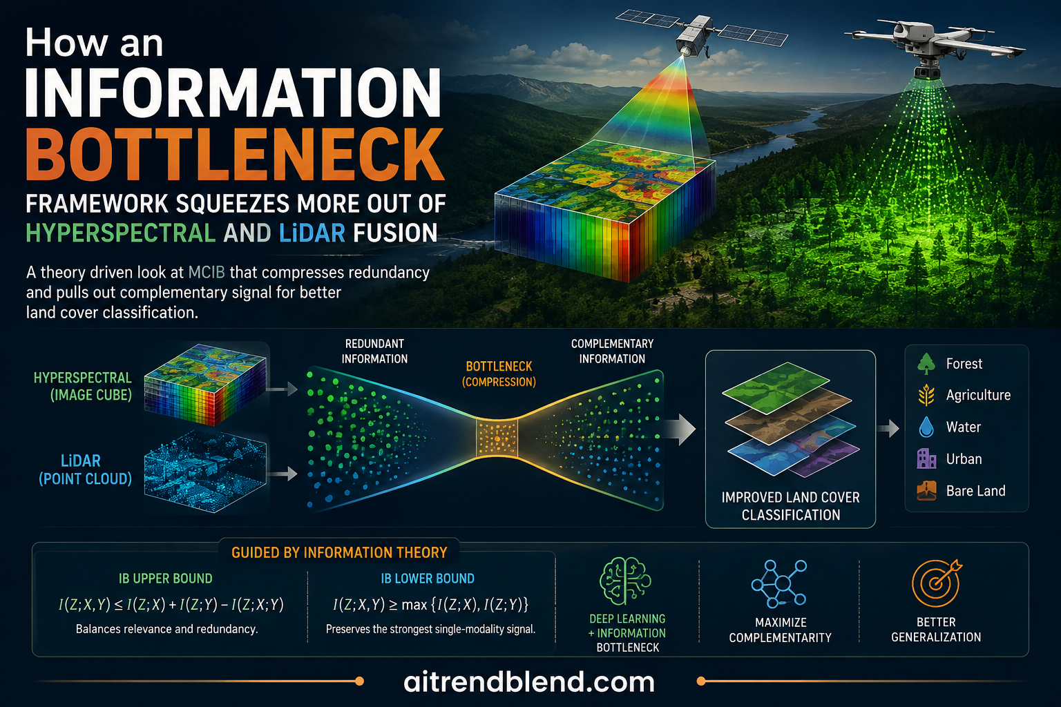
Picture a rooftop and a road sitting a few pixels apart in a satellite scene, both gray, both flat looking in a spectral plot, both the kind of thing that trips up a classifier trained on color alone. A sensor that only reads reflectance gets confused. A sensor that only reads height sees the answer immediately, because one of those surfaces sits three meters above the ground and the other does not. Researchers at Xidian University and Chang’an University spent this paper asking a fairly narrow but stubborn question. When you feed a model both kinds of data at once, hyperspectral imagery and LiDAR elevation, how do you make sure it actually uses the part of each source that the other one lacks, instead of just learning the same redundant shape twice.
Key points
- The paper introduces MCIB, a multimodal complementary information bottleneck framework for fusing hyperspectral imagery and LiDAR data in land use classification.
- It reframes the classic information bottleneck objective around joint mutual information terms rather than the sum of two separate unimodal ones, which changes what “redundant” and “sufficient” actually mean in a two sensor setting.
- Two theorems supply tractable upper and lower bounds so the joint objective, which is not directly computable, can still be optimized with ordinary gradient descent.
- A new contrastive loss called SCInfoNCE estimates the conditional mutual information terms that drive complementarity, and it reuses existing encoder and decoder components instead of adding a separate auxiliary network.
- On the Houston 2013, MUUFL Gulfport, and Trento benchmarks, MCIB reaches overall accuracy of 93.53 percent, 92.75 percent, and 93.34 percent respectively, ahead of eight comparison methods including recent transformer and contrastive approaches.
- The ablation study shows that redundancy compression alone gets you partway there, and that the complementarity term is responsible for most of the final gain, particularly on spectrally confusable classes like healthy grass versus stressed grass.
The problem hiding inside multimodal fusion
Land use and land cover classification is one of those tasks that sounds simple until you try to do it well. You want to label every pixel in a scene as water, road, building, grass, or one of a dozen other categories, and you want that label to hold up across shadows, seasons, and sensor noise. Hyperspectral imagery does a lot of that work on its own, since it reads reflectance across hundreds of narrow spectral bands and can tell a species of grass from a patch of dry soil that would look identical in an ordinary photograph. LiDAR data does something entirely different. It measures the timing of a laser pulse bouncing off a surface, which hands you elevation and structure rather than color. A road and a rooftop with a similar chemical composition will produce nearly the same spectral signature but wildly different heights.
The obvious move is to combine the two. Plenty of papers already do this, stacking features from separate branches, running cross attention between modalities, or training coupled convolutional networks that share parameters. The authors argue that most of this work is empirical rather than principled. Fusion architectures get built by trial and error, and while they often work, nobody can say with any rigor whether the model is actually extracting the complementary signal each sensor offers, or whether it is just burning capacity encoding the same shared information twice.
That distinction, between information that is shared and therefore redundant, and information that is unique to one modality and therefore valuable, is the entire premise of this paper. The authors point to two separate failure modes in existing multimodal methods. First, high correlation within each sensor’s own data, hundreds of adjacent hyperspectral bands that mostly say the same thing, or repetitive LiDAR geometry across a flat parking lot, means a lot of what gets encoded is simply noise or duplication. Second, and more interesting, most fusion objectives never explicitly ask the model to find the unique predictive power one modality offers exactly where the other one is ambiguous. They optimize for accuracy and hope complementarity emerges as a side effect.
Where the information bottleneck principle comes in
The information bottleneck principle, first formalized by Naftali Tishby, Fernando Pereira, and William Bialek around the turn of the century, gives a clean way to think about representation learning. You want a compressed representation Z of an input X that keeps as little information about X as possible while keeping as much information as possible about a target Y. Squeeze out the irrelevant noise, keep the signal that predicts the label. It has been applied across single modality settings for years, including a deep variational version from Alex Alemi and colleagues that made the objective tractable with neural networks through variational bounds.
Extending that idea to two sensors at once turns out to be less obvious than it sounds. A naive approach applies the standard bottleneck separately to each modality, compressing hyperspectral features on their own and LiDAR features on their own, then fusing the results. The paper argues this treats the two inputs as independent information sources and never models their joint distribution, which means it cannot guarantee that redundancy between the two branches actually gets removed, and it has no mechanism at all for pushing the model toward complementary information specifically.
What MCIB actually optimizes
The framework’s core move is to replace the sum of two separate bottleneck terms with two joint terms. Instead of minimizing the mutual information between each input and its own representation separately, MCIB minimizes the joint mutual information between both inputs together and both representations together, written as I of X_H, X_L with Z_H, Z_L. Instead of maximizing the sum of two separate sufficiency terms, it maximizes the joint mutual information between both representations and the label Y at once.
Why does that distinction matter in practice. Consider a building rooftop that both hyperspectral and LiDAR data can identify correctly on their own, since it has a distinctive spectral signature and a distinctive height. A model minimizing unimodal redundancy for each branch separately will happily let both Z_H and Z_L encode that shared fact in full, because from either branch’s own point of view nothing there looks redundant. Only when you look at the joint representation does the duplication become visible. The paper’s claim is that this overlooked overlap eats into the model’s effective capacity for encoding the information that is genuinely unique to each source, which is exactly the information a fusion system exists to extract.
The full MCIB objective is a Lagrangian trade off between joint compactness and joint sufficiency, controlled by a weighting parameter beta.
Both terms in that expression involve joint distributions across the two modalities and are not something you can compute directly with a neural network. This is where the paper’s two theorems earn their keep.
Theorem one, bounding the compactness term
To make the joint compactness term tractable, the authors introduce what they call an intra modal independence prior, essentially assuming each modality specific encoder only looks at its own input. That assumption lets them show, through a chain of mutual information identities, that the joint compactness term is bounded above by the sum of the two unimodal compression terms adjusted by a correction that involves the sufficiency terms for each modality and the joint sufficiency term. The gap between the true objective and this upper bound turns out to be exactly the conditional mutual information between the two representations given the label, a quantity that captures task irrelevant redundancy the two branches still share once you already know the correct category. Minimizing the upper bound pushes that gap toward zero, which is the theoretical ideal where each representation captures a genuinely distinct slice of what matters for the task.
Theorem two, bounding the sufficiency term
The second theorem tackles joint sufficiency from the other direction. Rather than trying to maximize I of Z_H, Z_L with Y directly, which again involves an intractable joint distribution, the authors expand it using the chain rule for mutual information into two equivalent decompositions, then take a weighted average controlled by a second parameter alpha. The key theoretical step replaces a conditional mutual information term involving the latent representation of one modality with the same term conditioned on the raw input of that modality instead, which is a looser but computable quantity, and a legitimate lower bound as long as each modality’s encoder is close to a sufficient statistic for its own input.
Those two conditional terms, the amount LiDAR representation Z_L tells you about the label given that you already know the full hyperspectral input, and the mirror image for Z_H given X_L, are the paper’s operational definition of complementarity. If Z_L still carries useful predictive signal even after conditioning on everything the hyperspectral sensor saw, that signal has to be coming from somewhere LiDAR uniquely contributes. Maximizing those terms is a direct, mathematically grounded way of asking the model to go find the information one sensor has and the other does not.
Why this framing matters
A lot of multimodal papers claim their fusion mechanism captures complementary information because the accuracy number went up. This paper instead defines complementarity as a specific conditional mutual information quantity, derives a bound for it, and builds a loss function that targets that quantity directly. The accuracy gain becomes evidence for the theory rather than a stand in for it.
Turning theory into a trainable network
Substituting both bounds back into the original Lagrangian gives a five term objective that splits cleanly into two jobs. The first two terms handle each modality’s own compression and sufficiency trade off and get optimized with the standard deep variational information bottleneck loss, which uses a KL divergence term to keep the latent representation close to a simple Gaussian prior and a log likelihood term through an auxiliary decoder to keep it predictive of the label. The last two terms handle the cross modal complementarity piece and require a way to estimate conditional mutual information, which is where the paper’s other main contribution shows up.
SCInfoNCE, contrastive learning built for a supervised setting
Standard InfoNCE, the contrastive estimator behind a lot of modern representation learning, works by scoring a positive pairing against a batch of negative pairings and training a critic to tell them apart. Estimating conditional mutual information specifically, rather than plain mutual information, usually requires an extra auxiliary distribution to generate negative samples that respect the conditioning variable. Sordoni and colleagues proposed one such conditional InfoNCE estimator, but it needs that additional variational component trained on the side.
The authors’ supervised conditional InfoNCE loss avoids adding anything new. It reuses the encoder and decoder that already exist for the deep variational bottleneck. To generate a negative label for a given hyperspectral sample, the network samples a latent Z_H from its own encoder, then samples a predicted label from the decoder trained on that same encoder. That predicted label distribution stands in for the conditional distribution of the label given the input, without training a separate network to model it. For each anchor sample the loss then pulls the LiDAR representation toward the true label given that context, while pushing it away from label predictions sampled from other, differently labeled examples. It is a fairly elegant piece of engineering, since it turns components the model already needs into the machinery for a harder estimation problem.
Network architecture in plain terms
The full pipeline runs two parallel branches. The hyperspectral branch uses a feature extractor built from ConvLSTM layers followed by convolutional blocks, since ConvLSTM handles the sequential structure across hundreds of spectral bands reasonably well. The LiDAR branch uses a more conventional convolutional stack, since elevation data does not have that same band sequence structure. Both branches map their features to a mean and log variance, sample a 256 dimensional latent vector using the reparameterization trick from Kingma and Welling’s variational autoencoder work, and pass that latent through a small decoder that predicts the label for the deep variational bottleneck loss. Two critic networks, structured as multilayer perceptrons, implement the SCInfoNCE loss for each direction of complementarity. Finally the two latent vectors get concatenated into a 512 dimensional fused representation and passed to a classifier trained with ordinary cross entropy. Every piece of the auxiliary machinery, the decoders and the critics, exists to shape that fused representation during training, not to add parameters at inference time beyond what a normal two branch fusion network already needs.
How well it actually performs
The evaluation runs on three widely used benchmarks. Houston 2013 comes from the 2013 IEEE GRSS Data Fusion Contest, covering the University of Houston campus with 144 hyperspectral bands and a single LiDAR channel across 15 land cover classes. MUUFL Gulfport covers the University of Southern Mississippi’s Gulf Park campus with 64 spectral bands and 4 LiDAR channels across 11 classes. Trento is a smaller, simpler rural scene near Trento, Italy with 63 spectral bands, a single LiDAR channel, and just 6 classes.
Against a field of ten comparison methods, including classic baselines like random forests and support vector machines, and more recent deep learning approaches such as EndNet, AsFNet, ExViT, DSFT, UDFNet, and two contrastive learning methods called CCL and MCFT, MCIB comes out ahead on all three datasets.
| Dataset | Overall accuracy | Average accuracy | Kappa times 100 |
|---|---|---|---|
| Houston 2013 | 93.53% | 93.91% | 92.97 |
| MUUFL Gulfport | 92.75% | 92.39% | 90.39 |
| Trento | 93.34% | 97.68% | 98.93 |
The margin over the closest competitor is not enormous in every case, and the authors are upfront about that on the Trento dataset, where fewer classes and a simpler rural scene leave less room for a redundancy and complementarity focused method to show its advantage. The more telling results show up in specific confusable classes rather than the aggregate numbers. On Houston 2013, MCIB pushes accuracy on the stressed grass class to 98.08 percent, compared with 84.53 percent for MIViT, a comparison method that also uses mutual information principles but without the joint complementarity formulation. On the same dataset, a highway class that sits in a shadowed region prone to being misread as water due to hyperspectral illumination sensitivity gets classified correctly 94.40 percent of the time by MCIB, against 73.15 percent for MIViT. The authors attribute that specific gain to LiDAR’s illumination invariant structure being explicitly pulled out as complementary information, rather than getting drowned out by the correlated, shadow confused hyperspectral signal.
Takeaway
The biggest wins in this paper do not come from the easy classes where either sensor alone would already do fine. They come from the classes where hyperspectral and LiDAR disagree with each other, which is exactly the scenario the joint complementarity term was built to handle.
What the ablation study shows
The ablation experiments are arguably more informative than the leaderboard comparison, because they isolate what each theoretical piece actually contributes. A baseline model trained only with cross entropy loss, no information theoretic regularization at all, sets the floor. Adding only the auxiliary decoders for intra modal sufficiency, or only the KL divergence constraint for intra modal compactness, produces small improvements over that baseline but consistently underperforms a model using both together, which the authors call MIB, short for the unimodal version without the joint complementarity term. That confirms compactness and sufficiency need to be optimized jointly rather than in isolation, which is not a surprising finding on its own.
The more interesting result is the jump from MIB to the full MCIB model, which adds the SCInfoNCE complementarity loss on top. On Houston 2013 that step alone accounts for a 3.57 percentage point gain in overall accuracy, considerably larger than the gain from adding the unimodal bottleneck regularization in the first place. Similar jumps show up on the other two datasets. The t-SNE visualizations included in the paper back this up qualitatively, with feature clusters for spectrally similar classes like healthy grass and stressed grass staying tangled together under the MIB model and separating cleanly once the complementarity term gets added.
Takeaway
Redundancy compression by itself is a modest improvement. The complementarity term, the part of the paper grounded in Theorem 2, is doing most of the actual work in the final accuracy numbers.
Where this fits and where it falls short
Parameter efficiency is worth a mention too. The paper reports model sizes in kilobytes across the three datasets, and MCIB lands in a reasonable middle range, clearly smaller than MIViT and MCFT despite outperforming both. That is a point in favor of the framework’s principled design over adding raw capacity, though it is also true that IEEE benchmark comparisons like this one do not always reflect deployment constraints such as inference latency on satellite or airborne hardware, which the paper does not measure.
The authors are honest about the framework’s limits in their own conclusion. MCIB is built specifically for two modalities, and while they suggest extending it to three or more sensors is conceptually possible, they acknowledge it would require handling a combinatorial increase in conditional mutual information terms and multi source conditioning that the current derivation does not cover. That is a meaningful gap if the goal is eventually folding in something like synthetic aperture radar or multispectral time series alongside hyperspectral and LiDAR, which is an increasingly common setup in operational Earth observation pipelines.
There is also a quieter limitation buried in the SCInfoNCE mechanism itself. Because negative samples come from ancestral sampling through the model’s own encoder and decoder, the quality and diversity of those negatives depends on how well trained those components already are, which is likely to be weakest early in training and under small batch sizes. The authors flag this directly and point to memory bank style negative sampling as a possible fix in future work, which is the kind of engineering fix that has helped contrastive learning methods in other domains scale past similar bottlenecks.
Why this matters beyond the benchmark tables
Stepping back from the specific accuracy numbers, the more durable contribution here is conceptual. A fair amount of multimodal fusion research in remote sensing treats architecture design as the main lever, adding another attention layer or another branch and hoping performance follows. This paper instead argues that the objective function itself was underspecified in a way that architecture alone cannot fix, since summing two separate unimodal bottleneck losses simply does not target the quantity that actually matters for a two sensor system. Whether or not every reader buys the full theoretical apparatus, the empirical result that explicit conditional mutual information maximization outperforms two other supervised contrastive baselines focused on cross modal alignment, CCL and MCFT, is a useful data point for anyone building fusion systems for satellite or airborne sensor data.
Honest limitations
A few things worth keeping in mind before treating these results as settled. First, all three benchmark datasets are relatively small by modern deep learning standards, with training sets ranging from 819 to 2832 samples, so generalization to larger, noisier operational datasets remains untested in this paper. Second, the equality conditions in both theorems describe an idealized state that the paper itself frames as a target the optimization approaches rather than something the trained model provably reaches, so the bounds are guarantees on the objective’s structure, not guarantees on what a finite training run with finite data will actually achieve. Third, the comparison against MIViT and other mutual information based baselines is informative but the paper does not report statistical significance testing between the top methods beyond standard deviation across five runs, which is a common gap in this subfield rather than one specific to this paper. Fourth, the framework’s reliance on a fixed patch size, tuned here to 11 by 11 pixels, and hyperparameters alpha and beta that clearly shift depending on the dataset’s spectral richness, suggests some amount of per dataset tuning is needed before deployment on a new sensor pairing or geography.
Reproducing the core idea
Below is a simplified but complete PyTorch implementation covering the two modality specific variational encoders, the deep variational bottleneck loss, a simplified supervised conditional InfoNCE loss, the fusion classifier, a training loop, an evaluation function, and a smoke test on random dummy data shaped like small hyperspectral and LiDAR patches. It is meant for learning and experimentation, not a drop in replacement for the authors’ original codebase, which was not released alongside the paper.
Two honest caveats on the code above. The per anchor loop inside the SCInfoNCE function trades speed for clarity and would need vectorizing for a real dataset of any size. The gamma and beta values are illustrative rather than tuned, since the paper derives its actual values for alpha and beta from a grid search shown in its figures rather than stating fixed defaults suitable for arbitrary data.
Conclusion
The core achievement of this paper is not a new architecture in the usual sense. It is a redefinition of what the information bottleneck objective should even be asking for once you have two sensors instead of one, replacing a sum of unimodal terms with joint terms that actually account for the interaction between modalities, then backing that redefinition with two proven bounds rather than an intuition. That theoretical grounding is what separates MCIB from the broader pile of fusion papers that rely on architectural cleverness alone, and it is also what gives the ablation study its clearest signal, since the complementarity term contributes more to the final accuracy than the redundancy compression term does across all three benchmarks.
There is a conceptual shift worth naming directly. Most information bottleneck applications treat compression as the main event and prediction as a constraint to satisfy along the way. This paper effectively treats the interaction between two information sources as the main event, with compression and prediction both serving that interaction. Framed that way, the method reads less like an incremental improvement on deep variational bottleneck methods and more like an attempt to ask what the bottleneck principle should look like once you take seriously that most interesting sensing problems are not single modality problems to begin with.
Transferability is a reasonable question to ask, and the paper only gestures at it. The intra modal independence prior and the joint mutual information formulation do not appear to be specific to hyperspectral or LiDAR data in any deep way, which suggests the same bounds could plausibly transfer to other paired sensing problems that share the same redundancy and complementarity structure, medical imaging pairings like MRI and PET come to mind, or audio and video in speech recognition. None of that is tested here, and it would be a mistake to treat it as demonstrated rather than plausible.
The honest limitations are worth repeating rather than glossing over. The framework as written handles exactly two modalities, the theoretical guarantees describe an idealized equality condition the trained model only approximates, and the negative sampling mechanism inside SCInfoNCE depends on the quality of components that are themselves still being trained, which the authors flag as an open problem rather than a solved one. Future work pointed to in the paper, particularly extending the framework past two modalities and replacing ancestral sampling with a memory bank, both look like reasonable next steps rather than afterthoughts.
None of that undercuts what the paper does show. Land cover classification is a task where the difference between a spectrally confused pixel and a correctly labeled one often comes down to exactly the kind of complementary information this framework was built to chase, and the accuracy gains on the hardest, most ambiguous classes back that up more convincingly than the headline numbers do. For anyone building or evaluating fusion systems on paired remote sensing data, this is a paper worth reading past the abstract.
Frequently asked questions
What does MCIB stand for and what problem does it solve
MCIB stands for multimodal complementary information bottleneck. It is a framework for combining hyperspectral imagery and LiDAR data for land use classification, built around the idea that a fusion model should explicitly compress redundant information shared between the two sensors while explicitly maximizing the unique, complementary information each sensor contributes.
How is this different from applying the standard information bottleneck to each sensor separately
Applying the bottleneck separately treats hyperspectral and LiDAR as independent sources and optimizes a sum of two unimodal objectives. MCIB instead formulates joint mutual information terms across both inputs and both representations at once, which the authors show through two theorems is necessary to properly remove cross modal redundancy and target genuinely complementary information rather than information either sensor could already provide on its own.
What is SCInfoNCE and why does it avoid an auxiliary network
SCInfoNCE, short for supervised conditional InfoNCE, is a contrastive loss designed to estimate conditional mutual information terms that standard InfoNCE cannot handle directly. Rather than training a separate network to model the conditional label distribution needed for negative sampling, it reuses the existing modality specific encoder and decoder already present in the model, generating negative labels through ancestral sampling from those components.
Which datasets and methods does the paper compare against
The paper evaluates on the Houston 2013, MUUFL Gulfport, and Trento benchmark datasets. Comparison methods include classic approaches like random forests and support vector machines, and deep learning baselines including EndNet, AsFNet, ExViT, DSFT, UDFNet, CCL, MCFT, and MIViT, with MCIB reaching the highest overall accuracy on all three datasets.
Does the complementarity term or the redundancy compression term matter more for accuracy
Based on the paper’s ablation study, the complementarity term contributes more to the final accuracy gain. Adding intra modal redundancy compression alone produced modest improvements over a plain baseline, while adding the SCInfoNCE complementarity loss on top produced a considerably larger jump, for example a 3.57 percentage point gain in overall accuracy on the Houston 2013 dataset.
Can this framework extend beyond two sensors, such as adding radar data
The authors state this directly as future work rather than something the current paper demonstrates. They describe extending MCIB past two modalities as conceptually feasible but note it would require handling a combinatorial increase in conditional mutual information terms and multi source conditioning that the present derivation does not cover.
Read the full paper for the complete proofs, hyperparameter sweeps, and additional visualizations that could not all fit into this summary.
Xiao Pan, Hao Zhu, Bo Yang, Changzhe Jiao, Jie Feng, and Jinjian Wu. MCIB, Multi-Modal Complementary Information Bottleneck for Hyperspectral and LiDAR Classification. IEEE Transactions on Image Processing, volume 35, 2026, pages 3053 to 3068. Digital Object Identifier 10.1109/TIP.2026.3673954. This analysis is based on the published paper and an independent evaluation of its claims.