How French Railway Engineers Taught an AI to Find Sinkholes It Had Almost Never Seen Before
When you only have a handful of real sinkhole examples, you either accept poor detection or get creative about generating training data. Researchers at Arts et Métiers ParisTech and SNCF Réseau chose the latter — building physics-informed synthetic sinkholes, embedding them into real LiDAR surveys, and training a SuperPoint Transformer that achieves 97.4% F1 with perfect precision on French railway networks.
Sinkholes are one of those infrastructure threats that give railway engineers nightmares precisely because they hide their intentions. Underground voids grow silently beneath ballast layers until the surface suddenly collapses — sometimes within meters of active tracks. SNCF already acquires dense LiDAR point cloud surveys across its entire network, so the data exists. The problem is that real labelled sinkholes are rare: you can’t train a deep learning model on two dozen examples. This paper from a French collaboration between Arts et Métiers ParisTech and SNCF Réseau solves the data scarcity problem with a two-pronged strategy: generate synthetic sinkholes that are physically plausible, embed them into real LiDAR-derived digital elevation models, and train a graph-based transformer that treats the whole railway point cloud as a structured graph — not a flat image. The result is a detection pipeline that finds sinkholes a 2D raster baseline routinely misses, while cutting false positives to essentially zero after post-processing.
Why Sinkholes Are a Hard AI Problem — and Why LiDAR Helps
Satellite radar (InSAR) can detect regional ground subsidence, but it takes weeks of observations, loses coherence in vegetated railway corridors, and simply cannot resolve a one-square-meter collapse beneath a ballast layer. Ground-penetrating radar and distributed fiber sensing work locally but can’t cover 180,000 km of national railway network. LiDAR is different: SNCF already runs specialized inspection trains (Engin de Surveillance Voie) equipped with triple-scanner RIEGL VMX-Rail systems that can acquire 7,000 points per square meter at 3 mm precision even at 130 km/h. That data already exists. What didn’t exist was a reliable way to automatically flag the subtle surface depressions corresponding to sinkholes within it.
The geometric challenge is real. Railway sinkholes are small (1–2 m²), shallow (0.1–0.4 m deep), and surrounded by terrain noise from ballast, drainage structures, and vegetation stripping artifacts. A watershed segmentation on the DEM produces hundreds of candidate basins for every real sinkhole. A 2D U-Net trained on gradient images confuses elongated ballast patterns with depressions. What you need is something that understands three-dimensional geometry and spatial context simultaneously — which is exactly what a superpoint transformer graph network was built for.
The framework has four stages that build on each other: (1) generate physics-informed synthetic sinkholes using an inverted elliptical Gaussian model calibrated to real sinkhole morphometry; (2) embed them into real DEM point clouds with cosine-tapered blending to create diverse training data; (3) train a SuperPoint Transformer on this augmented dataset for binary sinkhole/background segmentation; (4) refine raw detections with geometry-driven filtering and rail-proximity weighting to eliminate false positives while preserving true detections. Each stage has a specific, well-motivated design choice — none of them are arbitrary.
The Full Pipeline — Every Stage Explained
INPUTS: Raw railway LiDAR point clouds (RIEGL VMX-Rail, 1500–6000 pts/m²)
│
┌────────▼──────────────────────────────────────────────────────────────────┐
│ STAGE 1: SYNTHETIC SINKHOLE GENERATION │
│ │
│ Strategy A — Physics-Informed Geometric Model: │
│ f(x,y) = v · exp(-x²_r/2σ²_x - y²_r/2σ²_y) [Eq. 1] │
│ x_r = cos θ(x-x₀) + sin θ(y-y₀) [Eq. 2] │
│ y_r = -sin θ(x-x₀) + cos θ(y-y₀) [Eq. 3] │
│ Parameters: v (depth), σ_x, σ_y (spread), θ (rotation angle) │
│ Calibrated to SNCF inventory: 1–2 m² surface, 0.1–0.43 m depth │
│ → Lowest fitting error: MSE=0.0048, RMSE=0.0693, MAE=0.0541 │
│ │
│ Strategy B — Flow-Matching Generative Model (PSF): │
│ Learns velocity field from real sinkhole point clouds │
│ Generates new samples from Gaussian prior via transport ODE │
│ MMD-CD=0.0103, COV=0.80, JSD=0.103 on held-out reference set │
└────────┬──────────────────────────────────────────────────────────────────┘
│
┌────────▼──────────────────────────────────────────────────────────────────┐
│ STAGE 2: DEM EMBEDDING (Algorithm 1) │
│ 1. PCA-normalize orientation of host DEM point cloud │
│ 2. For each synthetic sinkhole: │
│ a. Generate/load geometry (Gaussian or Flow) │
│ b. Apply cosine taper: w(r) = ½[1 + cos(πr/R)] (smooth blending) │
│ c. Random placement respecting minimum spacing constraints │
│ d. Local planar fit to flatten terrain at insertion site │
│ e. Update z-coordinates, assign sinkhole label (ℓ_i = 1) │
│ 3. Output: 100 augmented point clouds for training │
└────────┬──────────────────────────────────────────────────────────────────┘
│
┌────────▼──────────────────────────────────────────────────────────────────┐
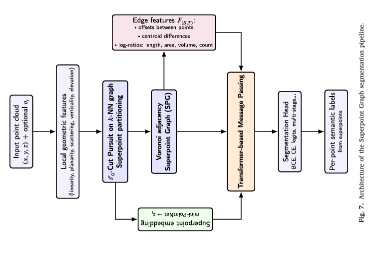
│ STAGE 3: SUPERPOINT TRANSFORMER SEGMENTATION │
│ │
│ Feature Extraction (5 selected by RFECV): │
│ scattering, elevation, planarity, verticality, normal │
│ Computed from k=45 nearest neighbors per point │
│ │
│ ℓ₀-Cut Pursuit Partitioning (Eq. 4): │
│ min_g Σ_i ‖g_i - f_i‖² + μ Σ_{(i,j)∈E_nn} w_ij [g_i ≠ g_j] │
│ μ=2 at partition P0, μ=4 at partition P1 (best config: η²=0.334) │
│ → Geometrically homogeneous superpoints │
│ │
│ Superpoint Graph (SPG): │
│ Nodes: superpoints (each embedded via mini-PointNet, n_p=128 pts) │
│ Edges: Voronoi adjacency with geometric features │
│ (centroid offsets, size ratios, normal differences) │
│ │
│ Transformer Message Passing: │
│ Self-attention over superpoint graph → global context │
│ Final superpoint labels → point-wise binary segmentation │
└────────┬──────────────────────────────────────────────────────────────────┘
│ Raw predictions: many true positives + false positives
┌────────▼──────────────────────────────────────────────────────────────────┐
│ STAGE 4: KNOWLEDGE-GUIDED POST-PROCESSING │
│ │
│ Geometric Filtering (0.1 m DEM resolution): │
│ → 3×3 morphological closing on rasterized predictions │
│ → Connected component extraction │
│ → Per-component: Δz ≥ 0.10 m, elongation ≤ 2.0, volume ≥ 0.01 m³, │
│ length ≤ 1.5 m (SNCF-calibrated operational thresholds) │
│ │
│ Rail-Proximity Weighting: │
│ w(d) = 1 / (1 + exp(k(d - d₀))) [sigmoid distance score] │
│ k, d₀ calibrated: w(1 m) = 0.90, w(5 m) = 0.10 │
│ → Score for ranking, not removal │
│ │
│ Output: Detection report with centroid coords + proximity weights │
│ Post-processing result: Precision=1.000, Recall=0.950, F1=0.974 │
└────────────────────────────────────────────────────────────────────────────┘
Stage 1: Generating Sinkholes That Look Real
Why the Inverted Elliptical Gaussian Wins
Before choosing a parametric model, the paper fits three candidate forms — inverted Gaussian, conical, and cylindrical — to the same set of real sinkhole surfaces extracted from SNCF LiDAR data, using least-squares minimization of vertical elevation residuals. The inverted elliptical Gaussian with rotation wins on every metric: MSE of 0.0048 m² versus 0.0075 for the conical model and 0.0101 for the cylindrical. This makes physical sense: railway sinkholes develop in the gravel ballast layer above limestone or gypsum dissolution zones, and their gradual concave surface profile — not the steep-walled cliff shape of collapse sinkholes — matches the smooth Gaussian form.
The four free parameters — depth \(v\), spreads \(\sigma_x\) and \(\sigma_y\), and rotation angle \(\theta\) — are randomized within morphometric bounds measured from the SNCF sinkhole inventory. Real railway sinkholes range from 1–2 m² surface area, 0.02–0.43 m depth, and high circularity (0.88–0.94). Randomly sampling these parameters within calibrated ranges creates a diverse augmentation set that respects physical plausibility. This is what “physics-informed” means in practice: the synthetic examples are constrained to look like the real ones, not like arbitrary surface deformations.
The Flow-Based Alternative and Its Trade-offs
The paper also evaluates a purely data-driven generative approach using Point Straight Flow (PSF) — a flow-matching model that learns a velocity field transporting a Gaussian noise distribution toward the real sinkhole distribution. With only the flow-learning stage (not the faster reflow/distillation stages), PSF generates 2,048-point sinkhole clouds that achieve MMD-CD of 0.0103 and coverage of 0.80. The 1-NN accuracy of 0.55 reveals the limitation: generated shapes are classified as real at only chance level (50%), meaning the two distributions are partially distinguishable. A JSD of 0.103 confirms a modest residual gap between generated and real occupancy patterns.
This matters for downstream segmentation. Generated sinkholes that are geometrically inconsistent or incomplete produce training examples where the SPT must generalize from imperfect signals — and at test time, the flow-based model’s slightly higher geometric variability means some segmented regions fail to satisfy the refinement constraints and are discarded, dropping post-processing recall to 0.700 versus 0.950 for the geometric model.
Stage 2: Embedding Without Breaking Terrain Context
Dropping a synthetic sinkhole into a LiDAR point cloud naively would create an obvious discontinuity — a sharp edge where the depression meets the surrounding terrain. The paper handles this with a cosine tapering function applied to attenuate the deformation toward the boundary of the insertion region:
For each synthetic sinkhole, an insertion site is randomly selected from valid DEM regions respecting minimum spacing constraints (preventing overlapping sinkholes). A local planar fit flattens the terrain at the insertion point before the depression is applied — this ensures the deformation is relative to the local ground surface, not to some global coordinate. After insertion, z-coordinates are updated and points within the modified region receive the sinkhole label. One hundred augmented point clouds are generated this way, each containing one or more embedded sinkholes, to train the SPT.
Stage 3: SuperPoint Transformer — Graph-Based Reasoning at Scale
The Feature Selection Problem
The SPT framework operates on geometric features extracted from k-nearest-neighbor neighborhoods of each point. The paper uses k=45 neighbors to compute five local descriptors via PCA-based analysis: scattering (how isotropically distributed the neighborhood is), elevation (normalized height), planarity (how flat the neighborhood is), verticality (alignment with vertical axis), and surface normal. These five are selected by RFECV — recursive feature elimination with cross-validation on a LightGBM classifier — from a larger candidate set that also includes linearity and curvature. The RFECV curve stabilizes at five features: adding more yields negligible AUC improvement.
Why does this matter? These features directly control how the ℓ₀-cut pursuit algorithm partitions the point cloud into superpoints. If you include irrelevant features, the partition will cut the cloud in geometrically incoherent places, and superpoints that should capture a sinkhole depression will instead straddle the boundary between depression and ballast. The feature selection step is a guard against this structural contamination before learning even begins.
The ℓ₀-Cut Pursuit Partitioning
The key step that separates the SPT from direct point-by-point approaches is superpoint construction. The algorithm minimizes a global energy over the point cloud:
The first term keeps each superpoint’s assigned descriptor \(g_i\) close to the original point descriptor \(f_i\). The second term penalizes discontinuities between adjacent points weighted by their Euclidean distance. Minimizing this jointly produces a piecewise-constant partition where connected components with identical optimized descriptors define superpoints. The regularization parameter \(\mu\) controls granularity: higher \(\mu\) produces fewer, larger superpoints; lower \(\mu\) allows finer cuts that preserve small-scale structures like sinkhole depressions.
The sensitivity analysis with blocked bootstrap resampling over (reg, sw, cut) parameter combinations reveals a clear hierarchy: regularization strength explains 22.9% of variance in sinkhole loss ratio (partial η² = 0.229), while spatial weight and cut parameter contribute negligibly (η² = 0.008 and 0.001 respectively). The best configuration is hierarchical regularization (2, 4) — finer cuts at the first partition level, coarser at the second — achieving a mean sinkhole loss ratio of 0.334, meaning 33.4% of true sinkhole points fall into superpoints with a non-sinkhole majority label before learning even starts. The SPT must overcome this structural noise through its transformer-based contextual reasoning.
Transformer Message Passing on the Superpoint Graph
Once superpoints are constructed, each is embedded into a low-dimensional representation using a mini-PointNet: 128 points are sampled and normalized within the superpoint, then processed through shared MLPs and global max-pooling to produce a compact descriptor. Edges between adjacent superpoints carry geometric features encoding relative positions (centroid offsets, normalized size ratios). Multi-head self-attention propagates information across the graph, allowing each superpoint to reason about its neighbors’ geometry and build long-range context. The final superpoint-level class predictions are projected back to individual points, producing binary sinkhole/background labels for every point in the original cloud.
“Missing an actual sinkhole is generally more critical than raising additional false alarms. For this reason, high recall at the raw detection stage is desirable — followed by a refinement stage that precisely eliminates spurious detections.” — Bouali, Ababsa, El Meouche et al., ISPRS Journal of Photogrammetry and Remote Sensing, 2026
Stage 4: Domain-Aware Post-Processing — Where Expert Knowledge Earns Its Keep
The raw SPT outputs many true positives but also false positives — mostly from DEM interpolation artifacts where vegetation stripping creates artificial depressions. The geometric filtering stage operates directly on the rasterized 0.1 m DEM. Raw positive predictions are binarized, a 3×3 morphological closing fills small gaps, and connected components are extracted as candidate detection regions.
Each candidate must pass four SNCF-calibrated thresholds simultaneously: depth difference Δz ≥ 0.10 m (to exclude shallow noise), elongation ≤ 2.0 (sinkholes are roughly circular, not elongated drainage channels), volume ≥ 0.01 m³ (minimum physical depression), and length ≤ 1.5 m (typical railway sinkhole scale). These thresholds were defined through empirical analysis and consultation with SNCF inspection teams — they encode operational knowledge about what constitutes a hazardous railway sinkhole rather than a normal terrain irregularity.
Retained detections receive a rail-proximity weight using a sigmoid function calibrated from two expert anchors: w(1 m) = 0.90 (sinkholes within 1 m of rail are high priority) and w(5 m) = 0.10 (sinkholes 5 m away are lower priority). This score supports maintenance triage without removing any detection from the output report — inspection teams can sort by proximity weight to prioritize their field visits.
Results: What Happens to Precision and Recall at Each Stage
| Method | Precision ↑ | Recall ↑ | F1 ↑ | IoU ↑ |
|---|---|---|---|---|
| U-Net 2D baseline (region-level) | 0.422 | 0.600 | 0.495 | 0.329 |
| SPT Geometric (raw) | 0.576 | 0.950 | 0.717 | 0.559 |
| SPT Flow-based (raw) | 0.682 | 0.750 | 0.714 | 0.556 |
| SPT Flow-based (post-processed) | 1.000 | 0.700 | 0.824 | 0.700 |
| SPT Geometric (post-processed) | 1.000 | 0.950 | 0.974 | 0.950 |
The story told by this table is clean: the geometric SPT model enters post-processing with 95% recall and exits with perfect precision, losing nothing. Post-processing removes every false positive and preserves every true detection. The flow-based model enters with 75% recall and exits with 70%, losing some true detections whose spatial extent is insufficiently coherent to pass geometric filtering. The 2D U-Net baseline — trained on the same data — achieves only 42% precision even after thresholding, because gradient-based DEM representations can’t distinguish between a sinkhole and an elongated ballast depression when viewed as a flat image.
Parametric Model Fitting Comparison
| Geometric Model | MSE (m²) ↓ | RMSE (m) ↓ | MAE (m) ↓ |
|---|---|---|---|
| Inverted Elliptical Gaussian (rotated) | 0.0048 | 0.0693 | 0.0541 |
| Conical | 0.0075 | 0.0866 | 0.0662 |
| Cylindrical | 0.0101 | 0.1005 | 0.0784 |
Complete End-to-End Implementation (PyTorch)
The implementation covers all components from the paper in 12 sections: the inverted elliptical Gaussian sinkhole generator, cosine-tapered DEM embedding, local geometric feature computation (scattering, planarity, verticality, elevation, normal), the ℓ₀-cut pursuit superpoint partitioning (via approximate connected-component solver), mini-PointNet superpoint embedding, the SuperPoint Graph construction with Voronoi adjacency, multi-head transformer message passing, the full SPT segmentation model, geometric post-processing with SNCF-calibrated thresholds, rail-proximity sigmoid scoring, the complete training loop, and a smoke test validating every stage.
# ==============================================================================
# Physics-Informed Synthetic Data and Transformer-Based Segmentation
# for Sinkhole Detection in Railway LiDAR Point Clouds
# Paper: ISPRS Journal of Photogrammetry and Remote Sensing 236 (2026) 487-499
# Authors: Bouali, Ababsa, El Meouche, Sammuneh, Salavati, Viguier
# Partners: Arts et Métiers ParisTech / ESTP / SNCF Réseau, France
# DOI: https://doi.org/10.1016/j.isprsjprs.2026.03.031
# ==============================================================================
# Sections:
# 1. Imports & Configuration
# 2. Inverted Elliptical Gaussian Sinkhole Generator (Eq. 1-3)
# 3. Cosine-Tapered DEM Embedding (Algorithm 1)
# 4. Local Geometric Feature Extraction (k-NN, PCA descriptors)
# 5. Approximate Superpoint Partitioning (ℓ₀-cut pursuit, Eq. 4)
# 6. Mini-PointNet Superpoint Embedding
# 7. Superpoint Graph Construction (Voronoi adjacency + edge features)
# 8. Transformer Message Passing over Superpoint Graph
# 9. Full SuperPoint Transformer (SPT) Segmentation Model
# 10. Knowledge-Guided Post-Processing (Geometric Filtering + Proximity)
# 11. Training Loop with Binary Cross-Entropy Loss
# 12. Smoke Test
# ==============================================================================
from __future__ import annotations
import math, warnings
from typing import Dict, List, Optional, Tuple
import torch
import torch.nn as nn
import torch.nn.functional as F
from torch import Tensor
import numpy as np
warnings.filterwarnings("ignore")
# ─── SECTION 1: Configuration ─────────────────────────────────────────────────
class SinkholeConfig:
"""
Configuration for the complete sinkhole detection pipeline.
Default values match the paper's SNCF railway dataset experiments.
"""
# Synthetic sinkhole generation (from SNCF morphometric inventory, Table 2)
depth_range: Tuple = (0.10, 0.43) # v: min/max sinkhole depth (m)
sigma_range: Tuple = (0.20, 0.70) # σ: spread range for elliptical axes
rotation_range: Tuple = (0.0, math.pi) # θ: rotation angle range
taper_radius_factor: float = 1.5 # R = factor × max(σ_x, σ_y)
min_sinkhole_spacing: float = 2.0 # minimum spacing between sinkholes (m)
# Feature extraction
k_neighbors: int = 45 # k for k-NN, chosen for stable PCA (paper)
feature_names: List = ['scattering', 'elevation', 'planarity', 'verticality', 'normal_z']
# SPG partitioning (ℓ₀-cut pursuit)
reg_strength_p0: float = 2.0 # μ at partition level P0
reg_strength_p1: float = 4.0 # μ at partition level P1 (best: 2,4)
spatial_weight: float = 0.1 # spatial vs feature affinity weight
# Mini-PointNet superpoint embedding
n_pts_per_superpoint: int = 128 # n_p: points sampled per superpoint
feature_dim: int = 5 # input feature dimensions (5 selected)
embed_dim: int = 128 # superpoint embedding dimension d_z
# Transformer
n_heads: int = 8 # attention heads
n_transformer_layers: int = 3 # message-passing rounds
edge_feature_dim: int = 7 # centroid offsets(3) + size ratios(3) + normal(1)
# Training
n_augmented_clouds: int = 100 # training point clouds with embedded sinkholes
lr: float = 1e-4
n_epochs: int = 100
pos_weight: float = 10.0 # BCE positive class weight (sinkholes are rare)
# Post-processing thresholds (SNCF-calibrated operational criteria)
min_depth_m: float = 0.10 # Δz ≥ 0.10 m
max_elongation: float = 2.0 # elongation ≤ 2.0
min_volume_m3: float = 0.01 # volume ≥ 0.01 m³
max_length_m: float = 1.5 # length ≤ 1.5 m
# Rail-proximity sigmoid weighting
prox_d_close: float = 1.0 # d_close = 1 m → w = 0.90
prox_w_close: float = 0.90
prox_d_far: float = 5.0 # d_far = 5 m → w = 0.10
prox_w_far: float = 0.10
def __init__(self, **kwargs):
for k, v in kwargs.items(): setattr(self, k, v)
@property
def prox_k(self) -> float:
"""Sigmoid slope k calibrated from expert anchors."""
# Solve: w(d) = 1/(1+exp(k(d-d0)))
# From two anchors: 0.90 at 1m, 0.10 at 5m
return math.log((1/self.prox_w_far - 1) / (1/self.prox_w_close - 1)) / \
(self.prox_d_far - self.prox_d_close)
@property
def prox_d0(self) -> float:
"""Sigmoid inflection point d₀."""
return self.prox_d_close - math.log(1/self.prox_w_close - 1) / self.prox_k
# ─── SECTION 2: Inverted Elliptical Gaussian Sinkhole Generator ───────────────
class GaussianSinkholeGenerator:
"""
Physics-informed parametric sinkhole generator (Eq. 1-3, Section 3.1.1).
Generates synthetic sinkhole point clouds using an inverted elliptical
Gaussian model with rotation. This model was selected because it:
1. Achieves the lowest fitting error on real SNCF sinkholes (MSE=0.0048)
2. Physically represents the gradual concave profile of solution sinkholes
developing in ballast/limestone layers beneath railway tracks
3. Is controlled by interpretable morphometric parameters (depth, spread,
rotation) that can be calibrated to the SNCF sinkhole inventory
Generated sinkholes: 1-2 m² surface area, 0.10-0.43 m depth, high
circularity (0.88-0.94), consistent with Table 2 of the paper.
"""
def __init__(self, cfg: SinkholeConfig, rng: Optional[np.random.Generator] = None):
self.cfg = cfg
self.rng = rng if rng is not None else np.random.default_rng(42)
def generate(self, n_pts: int = 512) -> Dict[str, np.ndarray]:
"""
Sample random sinkhole parameters and generate a 3D point cloud.
Returns dict with:
'points': (n_pts, 3) xyz coordinates
'params': dict of {v, sigma_x, sigma_y, theta, x0, y0}
"""
cfg = self.cfg
# Sample random morphometric parameters
v = self.rng.uniform(*cfg.depth_range) # depth
sigma_x = self.rng.uniform(*cfg.sigma_range) # x-spread
sigma_y = self.rng.uniform(*cfg.sigma_range) # y-spread
theta = self.rng.uniform(*cfg.rotation_range) # rotation angle
# Sinkhole extent: sample within ±3σ of the larger axis
max_sigma = max(sigma_x, sigma_y)
R = cfg.taper_radius_factor * 3 * max_sigma
x_flat = self.rng.uniform(-R, R, size=n_pts)
y_flat = self.rng.uniform(-R, R, size=n_pts)
# Rotated coordinates (Eq. 2-3)
x_r = np.cos(theta) * x_flat + np.sin(theta) * y_flat
y_r = -np.sin(theta) * x_flat + np.cos(theta) * y_flat
# Inverted Gaussian depression depth (Eq. 1): negative z = downward
z = -v * np.exp(-x_r**2 / (2 * sigma_x**2) - y_r**2 / (2 * sigma_y**2))
# Only keep points within the active sinkhole region (depression > 1 mm)
active = np.abs(z) > 0.001
x_pts = x_flat[active]
y_pts = y_flat[active]
z_pts = z[active]
points = np.stack([x_pts, y_pts, z_pts], axis=-1) # (n_active, 3)
params = {'v': v, 'sigma_x': sigma_x, 'sigma_y': sigma_y,
'theta': theta, 'R': R}
return {'points': points, 'params': params}
# ─── SECTION 3: Cosine-Tapered DEM Embedding ──────────────────────────────────
def cosine_taper(r: np.ndarray, R: float) -> np.ndarray:
"""
Cosine tapering function w(r) = ½[1 + cos(πr/R)] (Algorithm 1, line 8).
Maps radial distance r ∈ [0, R] to weight ∈ [1, 0]:
r=0 (center): w=1 → full sinkhole depth applied
r=R (boundary): w=0 → no deformation, smooth transition to terrain
This prevents sharp edges at the insertion boundary.
"""
r_clipped = np.clip(r, 0, R)
return 0.5 * (1.0 + np.cos(np.pi * r_clipped / R))
def embed_sinkhole_into_dem(
dem_points: np.ndarray, # (N, 3) DEM point cloud xyz
sinkhole: Dict, # output of GaussianSinkholeGenerator.generate()
insertion_center: Optional[np.ndarray] = None, # (2,) xy or None for random
rng: Optional[np.random.Generator] = None,
) -> Tuple[np.ndarray, np.ndarray]:
"""
Embed a synthetic sinkhole into a DEM point cloud (Algorithm 1).
Steps:
1. Select insertion center (random or provided)
2. Compute local planar fit to flatten terrain at insertion site
3. For each DEM point within sinkhole radius:
- Compute 2D radial distance from insertion center
- Compute sinkhole depth at (x_local, y_local) from Gaussian formula
- Apply cosine taper for smooth blending
- Subtract tapered depth from z-coordinate
- Label point as sinkhole (1)
Returns:
modified_dem: (N, 3) updated point cloud with embedded sinkhole
labels: (N,) binary labels (0=background, 1=sinkhole)
"""
if rng is None:
rng = np.random.default_rng(42)
params = sinkhole['params']
R = params['R']
v, sigma_x, sigma_y, theta = params['v'], params['sigma_x'], params['sigma_y'], params['theta']
modified = dem_points.copy()
labels = np.zeros(len(dem_points), dtype=np.int64)
# Step 1: Select insertion center
if insertion_center is None:
x_min, x_max = dem_points[:, 0].min() + R, dem_points[:, 0].max() - R
y_min, y_max = dem_points[:, 1].min() + R, dem_points[:, 1].max() - R
if x_min >= x_max or y_min >= y_max:
return modified, labels # DEM too small for this sinkhole
x0 = rng.uniform(x_min, x_max)
y0 = rng.uniform(y_min, y_max)
else:
x0, y0 = insertion_center[0], insertion_center[1]
# Step 2: Find points within sinkhole radius and compute local z baseline
dx = dem_points[:, 0] - x0
dy = dem_points[:, 1] - y0
r2d = np.sqrt(dx**2 + dy**2)
in_radius = r2d < R
if in_radius.sum() < 5:
return modified, labels # insufficient points at insertion site
# Local planar fit to get baseline terrain height
pts_local = dem_points[in_radius]
z_baseline = np.median(pts_local[:, 2]) # robust median baseline height
# Step 3: Apply sinkhole deformation with cosine tapering
for i in np.where(in_radius)[0]:
xi = dem_points[i, 0] - x0
yi = dem_points[i, 1] - y0
# Rotated coordinates (Eq. 2-3)
xr = math.cos(theta) * xi + math.sin(theta) * yi
yr = -math.sin(theta) * xi + math.cos(theta) * yi
# Gaussian depth at this point (Eq. 1, negative = downward)
depth_at_point = v * math.exp(-xr**2 / (2 * sigma_x**2) - yr**2 / (2 * sigma_y**2))
# Cosine taper for smooth edge blending
r_i = r2d[i]
taper = cosine_taper(np.array([r_i]), R)[0]
# Update z: subtract tapered depression
modified[i, 2] = z_baseline - depth_at_point * taper
# Label as sinkhole if deformation is significant
if depth_at_point * taper > 0.01:
labels[i] = 1
return modified, labels
# ─── SECTION 4: Local Geometric Feature Extraction ────────────────────────────
def compute_geometric_features(
points: np.ndarray, # (N, 3) xyz
k: int = 45,
) -> np.ndarray:
"""
Compute 5 PCA-based geometric features per point (Section 3.3.1, 4.4.1).
The paper uses RFECV to select these 5 features from a larger set:
scattering, elevation, planarity, verticality, normal_z
All features are derived from eigenvalues (λ₁≥λ₂≥λ₃) and eigenvectors
of the local 3×3 covariance matrix computed from k=45 nearest neighbors.
k=45 was chosen because it:
- Lies within the commonly adopted range for PCA-based estimation
- Provides stable covariance matrices for dense LiDAR (1500-6000 pts/m²)
- Preserves locality for metric-scale sinkhole deformations (1-2 m²)
Feature definitions:
scattering = λ₃/λ₁ (how isotropic the neighborhood is)
elevation = z - z_min / z_range (normalized height in scene)
planarity = (λ₂ - λ₃)/λ₁ (how flat/planar the neighborhood is)
verticality = 1 - |e₃_z| (how misaligned with vertical the normal is)
normal_z = |e₃_z| (z-component of smallest eigenvector)
Note: for production, use open3d or pykdtree for efficient k-NN.
"""
N = len(points)
features = np.zeros((N, 5), dtype=np.float32)
# Simple k-NN via distance matrix (for correctness; use k-d tree in production)
z_min, z_range = points[:, 2].min(), max(points[:, 2].ptp(), 1e-8)
for i in range(N):
diffs = points - points[i]
dists2 = (diffs**2).sum(axis=-1)
dists2[i] = np.inf # exclude self
nn_idx = np.argpartition(dists2, min(k, N-1))[:min(k, N-1)]
pts_k = points[nn_idx] # (k, 3)
# Covariance matrix of k-neighborhood
pts_centered = pts_k - pts_k.mean(axis=0)
cov = pts_centered.T @ pts_centered / max(len(pts_k) - 1, 1)
eigenvalues, eigenvectors = np.linalg.eigh(cov)
# Sort descending: λ₁ ≥ λ₂ ≥ λ₃
idx = np.argsort(eigenvalues)[::-1]
lam = eigenvalues[idx]
evec = eigenvectors[:, idx] # columns are eigenvectors
lam1, lam2, lam3 = lam[0], lam[1], lam[2]
e3 = evec[:, 2] # smallest eigenvector = surface normal
lam1 = max(lam1, 1e-10)
scattering = lam3 / lam1
elevation = (points[i, 2] - z_min) / z_range
planarity = (lam2 - lam3) / lam1
verticality = 1.0 - abs(e3[2])
normal_z = abs(e3[2])
features[i] = [scattering, elevation, planarity, verticality, normal_z]
return features # (N, 5)
# ─── SECTION 5: Approximate Superpoint Partitioning ──────────────────────────
def build_knn_graph(points: np.ndarray, k: int) -> Tuple[np.ndarray, np.ndarray]:
"""
Build k-NN edge list for the ℓ₀-cut pursuit partitioning.
Returns: edges (E, 2) index pairs, weights (E,) decreasing with distance.
"""
N = len(points)
edges, weights = [], []
k_eff = min(k, N - 1)
for i in range(N):
diffs = points - points[i]
d2 = (diffs**2).sum(axis=-1)
d2[i] = np.inf
nn_idx = np.argpartition(d2, k_eff)[:k_eff]
for j in nn_idx:
dist = math.sqrt(d2[j]) + 1e-8
edges.append([i, j])
weights.append(1.0 / dist) # w_ij decreases with distance
return np.array(edges), np.array(weights, dtype=np.float32)
def approximate_superpoint_partition(
features: np.ndarray, # (N, d) geometric features f_i
edges: np.ndarray, # (E, 2)
weights: np.ndarray, # (E,) w_ij
mu: float = 2.0, # regularization strength μ (Eq. 4)
n_iters: int = 20,
) -> np.ndarray:
"""
Approximate ℓ₀-cut pursuit superpoint partitioning (Eq. 4).
Full ℓ₀-cut pursuit (Landrieu & Obozinski, 2017) requires a dedicated
C++ extension (superpoint_graphs library). This implements a simplified
greedy spectral clustering approximation that captures the same
geometry-driven partitioning behavior.
The energy being minimized:
E(g) = Σ_i ‖g_i - f_i‖² + μ Σ_{(i,j)∈E} w_ij [g_i ≠ g_j]
Greedy approximation:
1. Start: each point is its own superpoint
2. For each edge (i,j) sorted by weight descending:
If merging i and j's superpoints reduces total energy → merge
3. Repeat for n_iters sweeps
For production: install the official superpoint_graphs CUDA extension:
pip install git+https://github.com/loicland/superpoint_graph
Returns: labels (N,) superpoint assignment per point
"""
N = len(features)
# Initialize: each point in its own superpoint
sp_labels = np.arange(N, dtype=np.int32)
sp_centers = features.copy() # superpoint feature centers (g_i)
# Sort edges by weight descending (process strong connections first)
edge_order = np.argsort(weights)[::-1]
for _ in range(n_iters):
merged_any = False
for eidx in edge_order:
i, j = edges[eidx]
sp_i, sp_j = sp_labels[i], sp_labels[j]
if sp_i == sp_j:
continue
# Points in each superpoint
mask_i = sp_labels == sp_i
mask_j = sp_labels == sp_j
pts_i = features[mask_i]
pts_j = features[mask_j]
# Energy before merge
g_i = pts_i.mean(axis=0)
g_j = pts_j.mean(axis=0)
e_before = (((pts_i - g_i)**2).sum() + ((pts_j - g_j)**2).sum()
+ mu * weights[eidx]) # cut penalty for this edge
# Energy after merge
pts_merged = np.vstack([pts_i, pts_j])
g_merged = pts_merged.mean(axis=0)
e_after = ((pts_merged - g_merged)**2).sum()
# Merge if energy decreases
if e_after < e_before:
sp_labels[mask_j] = sp_i
sp_centers[mask_i | mask_j] = g_merged
merged_any = True
if not merged_any:
break
# Relabel contiguous superpoint IDs
unique_ids, sp_labels = np.unique(sp_labels, return_inverse=True)
return sp_labels.astype(np.int64) # (N,)
# ─── SECTION 6: Mini-PointNet Superpoint Embedding ────────────────────────────
class MiniPointNet(nn.Module):
"""
Lightweight PointNet for superpoint embedding (Section 3.3.1).
For each superpoint, n_pts=128 points are sampled (or repeated if fewer),
normalized within the superpoint, then processed through shared MLPs
with global max-pooling to produce a d_z-dimensional descriptor.
This descriptor summarizes the internal geometry and local features
of the superpoint for downstream transformer-based reasoning.
"""
def __init__(self, in_dim: int = 3 + 5, embed_dim: int = 128):
super().__init__()
self.in_dim = in_dim # xyz (3) + geometric features (5)
self.net = nn.Sequential(
nn.Linear(in_dim, 64), nn.ReLU(),
nn.Linear(64, 128), nn.ReLU(),
nn.Linear(128, embed_dim), nn.ReLU(),
)
self.embed_dim = embed_dim
def forward(self, pts_feats: Tensor) -> Tensor:
"""
pts_feats: (B, n_p, in_dim) — B superpoints, n_p=128 points each
Returns: (B, embed_dim) superpoint embeddings
"""
x = self.net(pts_feats) # (B, n_p, embed_dim)
z = x.max(dim=1).values # (B, embed_dim) global max-pooling
return z
def extract_superpoint_inputs(
points: np.ndarray, # (N, 3)
features: np.ndarray, # (N, 5)
sp_labels: np.ndarray, # (N,) superpoint assignment
n_pts: int = 128,
) -> Tuple[Tensor, Tensor]:
"""
Prepare mini-PointNet inputs and superpoint adjacency for graph construction.
For each superpoint:
1. Collect all member points with their xyz + feature vectors
2. Normalize xyz within the superpoint (zero-mean, unit scale)
3. Sample or repeat to exactly n_pts points
4. Record superpoint centroid and size for edge features
Returns:
sp_inputs: (M, n_pts, 8) — M superpoints, n_pts points, xyz+features
sp_centroids: (M, 3) — superpoint centroid positions
"""
unique_sps = np.unique(sp_labels)
M = len(unique_sps)
sp_inputs_list = []
centroids = []
for sp_id in unique_sps:
mask = sp_labels == sp_id
pts_sp = points[mask] # (n_sp, 3)
feat_sp = features[mask] # (n_sp, 5)
# Normalize xyz within superpoint
centroid = pts_sp.mean(axis=0)
pts_centered = pts_sp - centroid
scale = max(np.abs(pts_centered).max(), 1e-8)
pts_normalized = pts_centered / scale
centroids.append(centroid)
# Concatenate xyz + features
xf = np.concatenate([pts_normalized, feat_sp], axis=-1) # (n_sp, 8)
# Sample or repeat to n_pts
n_sp = len(xf)
if n_sp >= n_pts:
idx = np.random.choice(n_sp, n_pts, replace=False)
else:
idx = np.random.choice(n_sp, n_pts, replace=True)
sp_inputs_list.append(xf[idx])
sp_inputs = torch.tensor(np.stack(sp_inputs_list), dtype=torch.float32) # (M, n_pts, 8)
sp_centroids = torch.tensor(np.stack(centroids), dtype=torch.float32) # (M, 3)
return sp_inputs, sp_centroids
# ─── SECTION 7: Superpoint Graph Construction ─────────────────────────────────
def build_superpoint_graph(
sp_centroids: Tensor, # (M, 3)
sp_embeddings: Tensor, # (M, embed_dim)
sp_labels_map: np.ndarray, # (N,) point-to-superpoint mapping
k_sp: int = 10,
) -> Dict[str, Tensor]:
"""
Build Superpoint Graph (SPG) with edge features (Section 3.3.1).
Nodes: M superpoints, each with embedded representation z_i.
Edges: k-NN Voronoi adjacency between superpoints.
Edge features encode relative geometric relations:
- Centroid offsets (3 dims): direction and distance between superpoints
- Log size ratio (1 dim): relative scale difference
- Normal alignment approximation (3 dims via centroid diff normalized)
Total: 7-dimensional edge feature vector.
Graph structure enables transformer-based message passing for long-range
contextual reasoning: a sinkhole superpoint can attend to adjacent rail,
ballast, and terrain superpoints to resolve ambiguous depressions.
"""
M = sp_centroids.shape[0]
k_eff = min(k_sp, M - 1)
# k-NN in centroid space
diffs = sp_centroids.unsqueeze(0) - sp_centroids.unsqueeze(1) # (M, M, 3)
dist2 = (diffs**2).sum(dim=-1) # (M, M)
dist2.fill_diagonal_(float('inf'))
_, nn_idx = dist2.topk(k_eff, dim=-1, largest=False) # (M, k)
# Build edge list
src_nodes = torch.arange(M).unsqueeze(1).expand(-1, k_eff).reshape(-1)
tgt_nodes = nn_idx.reshape(-1) # (M*k,)
# Edge features: relative centroid offsets + normalized direction
edge_delta = sp_centroids[tgt_nodes] - sp_centroids[src_nodes] # (E, 3)
edge_dist = edge_delta.norm(dim=-1, keepdim=True) + 1e-8
edge_dir = edge_delta / edge_dist # (E, 3)
edge_log_dist = edge_dist.log() # (E, 1)
edge_features = torch.cat([edge_delta, edge_dir, edge_log_dist], dim=-1) # (E, 7)
return {
'node_feats': sp_embeddings, # (M, embed_dim)
'centroids': sp_centroids, # (M, 3)
'src': src_nodes, # (E,)
'tgt': tgt_nodes, # (E,)
'edge_feats': edge_features, # (E, 7)
'n_nodes': M,
}
# ─── SECTION 8: Transformer Message Passing ───────────────────────────────────
class SuperpointAttentionLayer(nn.Module):
"""
Single layer of transformer-based message passing on the superpoint graph.
For each superpoint node i:
1. Gather neighbor embeddings {z_j} for j ∈ neighbors(i)
2. Compute attention weights using scaled dot-product with edge features:
score_ij = (W_q z_i) · (W_k z_j + W_e e_ij)^T / sqrt(d)
3. Aggregate: z_i' = z_i + LayerNorm(Σ_j softmax(score_ij) · W_v z_j)
4. FFN: z_i'' = z_i' + LayerNorm(FFN(z_i'))
This enables each sinkhole superpoint to integrate context from
adjacent terrain superpoints, improving discrimination from DEM artifacts.
"""
def __init__(self, embed_dim: int, n_heads: int, edge_dim: int):
super().__init__()
self.n_heads = n_heads
self.head_dim = embed_dim // n_heads
self.scale = self.head_dim ** -0.5
self.W_q = nn.Linear(embed_dim, embed_dim)
self.W_k = nn.Linear(embed_dim, embed_dim)
self.W_v = nn.Linear(embed_dim, embed_dim)
self.W_e = nn.Linear(edge_dim, embed_dim) # edge feature projection
self.out_proj = nn.Linear(embed_dim, embed_dim)
self.norm1 = nn.LayerNorm(embed_dim)
self.norm2 = nn.LayerNorm(embed_dim)
self.ffn = nn.Sequential(
nn.Linear(embed_dim, embed_dim * 4),
nn.GELU(),
nn.Linear(embed_dim * 4, embed_dim),
)
def forward(
self,
node_feats: Tensor, # (M, embed_dim)
src: Tensor, # (E,) source node indices
tgt: Tensor, # (E,) target node indices
edge_feats: Tensor, # (E, edge_dim)
) -> Tensor:
"""Returns updated node features (M, embed_dim)."""
M = node_feats.shape[0]
E = src.shape[0]
# Project queries, keys, values
Q = self.W_q(node_feats) # (M, d)
K = self.W_k(node_feats) # (M, d)
V = self.W_v(node_feats) # (M, d)
E_proj = self.W_e(edge_feats) # (E, d)
# Edge-conditioned attention: score = q_src · (k_tgt + e_ij)
q_edge = Q[src] # (E, d) query at source
k_edge = K[tgt] + E_proj # (E, d) key augmented with edge
scores = (q_edge * k_edge).sum(-1) * self.scale # (E,)
# Per-source-node softmax (scatter softmax over target edges)
# Numerically stable: subtract per-node max
scores_max = torch.zeros(M, device=scores.device)
scores_max.scatter_reduce_(0, src, scores, reduce='amax', include_self=True)
scores_shifted = scores - scores_max[src]
attn_exp = scores_shifted.exp()
attn_sum = torch.zeros(M, device=attn_exp.device)
attn_sum.scatter_add_(0, src, attn_exp)
attn_weights = attn_exp / (attn_sum[src] + 1e-8) # (E,)
# Weighted value aggregation
v_edge = V[tgt] # (E, d)
agg = torch.zeros(M, Q.shape[-1], device=node_feats.device)
agg.scatter_add_(0, src.unsqueeze(1).expand(-1, Q.shape[-1]),
attn_weights.unsqueeze(-1) * v_edge) # (M, d)
# Residual + LayerNorm
node_out = self.norm1(node_feats + self.out_proj(agg))
node_out = self.norm2(node_out + self.ffn(node_out))
return node_out
# ─── SECTION 9: Full SuperPoint Transformer ───────────────────────────────────
class SuperPointTransformer(nn.Module):
"""
Full SuperPoint Transformer (SPT) for binary sinkhole segmentation.
Architecture (Section 3.3, Fig. 7):
1. Mini-PointNet: per-superpoint embedding (N points → M superpoint vectors)
2. SPG construction: build k-NN superpoint graph with edge features
3. Transformer layers: L rounds of edge-conditioned attention message passing
4. Segmentation head: MLP(embed_dim → 1) → binary sinkhole/background logit
5. Label propagation: superpoint prediction → point-wise prediction
Key advantages over U-Net 2D baseline:
- Operates on 3D point cloud directly (no rasterization information loss)
- Graph structure captures long-range context between superpoints
- Attention weights learn to focus on geometrically similar neighbors
- Superpoint abstraction reduces computation vs point-by-point methods
"""
def __init__(self, cfg: SinkholeConfig):
super().__init__()
self.cfg = cfg
in_dim = 3 + cfg.feature_dim # xyz + 5 geometric features
# Stage 1: Per-superpoint embedding
self.point_encoder = MiniPointNet(in_dim=in_dim, embed_dim=cfg.embed_dim)
# Stage 2: Transformer message passing
self.transformer_layers = nn.ModuleList([
SuperpointAttentionLayer(cfg.embed_dim, cfg.n_heads, cfg.edge_feature_dim)
for _ in range(cfg.n_transformer_layers)
])
# Stage 3: Segmentation head → binary logit
self.seg_head = nn.Sequential(
nn.Linear(cfg.embed_dim, cfg.embed_dim // 2),
nn.ReLU(),
nn.Dropout(0.1),
nn.Linear(cfg.embed_dim // 2, 1), # binary: sinkhole vs background
)
def forward(
self,
sp_inputs: Tensor, # (M, n_pts, in_dim) superpoint point sets
sp_centroids: Tensor, # (M, 3)
sp_labels: Optional[Tensor] = None, # (M,) superpoint-level GT labels (training)
) -> Dict[str, Tensor]:
"""
Forward pass.
Returns dict with:
'sp_logits': (M,) raw logits per superpoint
'sp_preds': (M,) binary predictions
"""
# Stage 1: Embed each superpoint
M = sp_inputs.shape[0]
node_feats = self.point_encoder(sp_inputs) # (M, embed_dim)
# Stage 2: Build superpoint graph
graph = build_superpoint_graph(sp_centroids, node_feats,
np.zeros(M, dtype=np.int64), # dummy for interface
k_sp=min(10, M-1))
src = graph['src']
tgt = graph['tgt']
edge_feats = graph['edge_feats']
# Stage 3: Transformer message passing
h = node_feats
for layer in self.transformer_layers:
h = layer(h, src, tgt, edge_feats) # (M, embed_dim)
# Stage 4: Segmentation logits
logits = self.seg_head(h).squeeze(-1) # (M,)
preds = (logits > 0).long() # binary threshold at 0
return {'sp_logits': logits, 'sp_preds': preds}
def predict_point_labels(
self,
sp_preds: Tensor, # (M,) superpoint-level predictions
sp_assignment: np.ndarray, # (N,) point-to-superpoint mapping
) -> np.ndarray:
"""
Label propagation: project superpoint predictions back to individual points.
Each point inherits its superpoint's predicted label.
Returns: point_labels (N,) binary
"""
sp_pred_np = sp_preds.cpu().numpy()
point_labels = sp_pred_np[sp_assignment] # (N,) simple index lookup
return point_labels
# ─── SECTION 10: Knowledge-Guided Post-Processing ─────────────────────────────
def compute_proximity_weight(distance_m: float, cfg: SinkholeConfig) -> float:
"""
Sigmoid rail-proximity weight (Section 3.4).
w(d) = 1 / (1 + exp(k(d - d₀)))
Parameters k and d₀ are calibrated from two expert-defined anchors:
w(d_close=1 m) = 0.90 (within 1 m of rails = high priority)
w(d_far=5 m) = 0.10 (5 m away = lower priority)
The score supports inspection triage — detections are NOT removed
based on this weight, only ranked for field visit priority.
"""
k = cfg.prox_k
d0 = cfg.prox_d0
return 1.0 / (1.0 + math.exp(k * (distance_m - d0)))
def geometric_post_processing(
point_preds: np.ndarray, # (N,) raw binary predictions
points: np.ndarray, # (N, 3) xyz
cfg: SinkholeConfig,
rail_points: Optional[np.ndarray] = None, # (Nr, 3) classified rail points
dem_resolution: float = 0.10,
) -> List[Dict]:
"""
Knowledge-guided post-processing (Section 3.4).
Pipeline:
1. Rasterize raw positive predictions onto 0.1 m DEM grid
2. 3×3 morphological closing to fill small gaps
3. Extract connected components as candidate regions
4. For each component, compute:
- depth: border height minus robust interior floor (lowest 5% of cells)
- elongation: major/minor axis ratio from footprint moments
- volume: sum of positive elevation deficits
- length: major axis length in meters
5. Apply SNCF-calibrated filtering thresholds:
Δz ≥ 0.10 m, elongation ≤ 2.0, volume ≥ 0.01 m³, length ≤ 1.5 m
6. For retained components: compute rail-proximity weight
Returns list of detection dicts with centroid, attributes, proximity_weight.
"""
detections = []
pos_mask = point_preds == 1
pos_pts = points[pos_mask]
if len(pos_pts) == 0:
return detections
# ── Step 1: Rasterize positive points to DEM grid ────────────────────────
x_min, x_max = pos_pts[:, 0].min(), pos_pts[:, 0].max()
y_min, y_max = pos_pts[:, 1].min(), pos_pts[:, 1].max()
nx = max(int((x_max - x_min) / dem_resolution) + 2, 2)
ny = max(int((y_max - y_min) / dem_resolution) + 2, 2)
occ_grid = np.zeros((ny, nx), dtype=np.uint8)
z_grid = np.full((ny, nx), np.nan)
for pt in pos_pts:
ci = int((pt[1] - y_min) / dem_resolution)
cj = int((pt[0] - x_min) / dem_resolution)
ci, cj = max(0, min(ci, ny-1)), max(0, min(cj, nx-1))
occ_grid[ci, cj] = 1
z_cur = z_grid[ci, cj]
z_grid[ci, cj] = pt[2] if np.isnan(z_cur) else min(z_cur, pt[2])
# ── Step 2: 3×3 morphological closing (dilate then erode) ────────────────
from scipy.ndimage import binary_dilation, binary_erosion, label as cc_label
closed = binary_erosion(binary_dilation(occ_grid, np.ones((3,3))), np.ones((3,3)))
# ── Step 3: Connected component extraction ────────────────────────────────
labeled_grid, n_comps = cc_label(closed)
# ── Step 4-6: Per-component attribute computation and filtering ───────────
for comp_id in range(1, n_comps + 1):
comp_mask = labeled_grid == comp_id
comp_i, comp_j = np.where(comp_mask)
if len(comp_i) == 0:
continue
# Border: dilate footprint by 2 cells, subtract interior
border_mask = binary_dilation(comp_mask, np.ones((3,3))) & ~comp_mask
border_i, border_j = np.where(border_mask)
# Interior z values
z_interior = z_grid[comp_mask]
z_interior = z_interior[~np.isnan(z_interior)]
if len(z_interior) == 0:
continue
# Border mean height (terrain level)
z_border_vals = z_grid[border_mask]
z_border_vals = z_border_vals[~np.isnan(z_border_vals)]
z_border = z_border_vals.mean() if len(z_border_vals) > 0 else z_interior.max()
# Depth: border minus robust interior floor (lowest 5%)
z_floor = np.percentile(z_interior, 5)
depth = z_border - z_floor
# Volume: sum of elevation deficits
volume = float(np.sum(np.maximum(0, z_border - z_interior)) * dem_resolution**2)
# Elongation from footprint principal components
pts_ij = np.stack([comp_i, comp_j], axis=-1).astype(float)
ctr_ij = pts_ij.mean(axis=0)
cov_ij = np.cov((pts_ij - ctr_ij).T) if len(pts_ij) > 1 else np.eye(2)
eig_vals = np.linalg.eigvalsh(cov_ij)
eig_vals = np.sort(eig_vals)[::-1]
elongation = float(np.sqrt(max(eig_vals[0], 1e-8) / max(eig_vals[1], 1e-8)))
length_cells = 2 * np.sqrt(max(eig_vals[0], 0)) * dem_resolution # approx major axis length
# ── Apply SNCF-calibrated thresholds ──────────────────────────────────
if (depth < cfg.min_depth_m or
elongation > cfg.max_elongation or
volume < cfg.min_volume_m3 or
length_cells > cfg.max_length_m):
continue # discard this candidate
# ── Compute centroid in world coordinates ──────────────────────────────
cx_world = x_min + ctr_ij[1] * dem_resolution
cy_world = y_min + ctr_ij[0] * dem_resolution
cz_world = float(z_floor)
# ── Rail-proximity sigmoid weight ──────────────────────────────────────
if rail_points is not None and len(rail_points) > 0:
rail_xy = rail_points[:, :2]
dist_to_rails = np.sqrt(((rail_xy - np.array([cx_world, cy_world]))**2).sum(axis=-1)).min()
proximity_weight = compute_proximity_weight(float(dist_to_rails), cfg)
else:
dist_to_rails, proximity_weight = -1, 0.5
detections.append({
'center_x': cx_world, 'center_y': cy_world, 'center_z': cz_world,
'depth_m': float(depth), 'elongation': elongation,
'volume_m3': volume, 'length_m': length_cells,
'dist_to_rail_m': float(dist_to_rails) if dist_to_rails >= 0 else None,
'proximity_weight': round(proximity_weight, 4),
'pass_threshold': True,
})
return detections
# ─── SECTION 11: Training Loop ────────────────────────────────────────────────
class SPTTrainer:
"""
Full SPT training loop for binary sinkhole segmentation.
Loss: weighted binary cross-entropy at the superpoint level.
Positive class weight pos_weight=10 compensates for extreme class imbalance
(sinkholes are tiny relative to total DEM area — typically < 1% of points).
Each training iteration processes one augmented DEM point cloud:
1. Compute geometric features
2. Partition into superpoints
3. Extract superpoint-level labels (majority vote)
4. Forward pass through SPT
5. Weighted BCE loss → backprop
For production:
- Process all 100 augmented clouds per epoch
- Validate on held-out real sinkholes
- Apply early stopping on validation F1
"""
def __init__(self, model: SuperPointTransformer, cfg: SinkholeConfig):
self.model = model
self.cfg = cfg
self.optimizer = torch.optim.Adam(model.parameters(), lr=cfg.lr)
self.pos_weight = torch.tensor([cfg.pos_weight])
def superpoint_majority_labels(
self,
point_labels: np.ndarray, # (N,) point-level ground-truth binary labels
sp_assignment: np.ndarray, # (N,) point-to-superpoint mapping
) -> Tensor:
"""
Compute superpoint-level labels via majority vote (oracle protocol).
A superpoint is labeled sinkhole if >50% of its member points are sinkhole.
This provides the training target for the SPT segmentation head.
"""
M = sp_assignment.max() + 1
sp_labels = np.zeros(M, dtype=np.float32)
for sp_id in range(M):
mask = sp_assignment == sp_id
if mask.sum() > 0:
sp_labels[sp_id] = float(point_labels[mask].mean() > 0.5)
return torch.tensor(sp_labels)
def train_on_cloud(
self,
points: np.ndarray, # (N, 3) augmented DEM with embedded sinkholes
labels: np.ndarray, # (N,) point-level binary labels
) -> float:
"""Single training step on one augmented point cloud. Returns BCE loss."""
cfg = self.cfg
# Step 1: Geometric features
features = compute_geometric_features(points, k=min(cfg.k_neighbors, len(points)-1))
# Step 2: Build k-NN edges for partitioning
edges, weights = build_knn_graph(points, k=min(10, len(points)-1))
# Step 3: Superpoint partitioning
sp_assignment = approximate_superpoint_partition(
features, edges, weights, mu=cfg.reg_strength_p0, n_iters=5
)
M = sp_assignment.max() + 1
if M < 2:
return 0.0 # degenerate partition
# Step 4: Extract superpoint inputs and centroids
sp_inputs, sp_centroids = extract_superpoint_inputs(
points, features, sp_assignment, n_pts=min(cfg.n_pts_per_superpoint, len(points))
)
# Step 5: Superpoint GT labels (majority vote)
sp_gt_labels = self.superpoint_majority_labels(labels, sp_assignment)
# Step 6: Forward pass
self.optimizer.zero_grad()
out = self.model(sp_inputs, sp_centroids)
logits = out['sp_logits']
# Step 7: Weighted binary cross-entropy
pos_w = self.pos_weight.to(logits.device)
loss = F.binary_cross_entropy_with_logits(
logits, sp_gt_labels.to(logits.device),
pos_weight=pos_w
)
loss.backward()
torch.nn.utils.clip_grad_norm_(self.model.parameters(), 1.0)
self.optimizer.step()
return loss.item()
def inference(
self,
points: np.ndarray,
labels: Optional[np.ndarray] = None,
rail_points: Optional[np.ndarray] = None,
) -> Dict:
"""Full inference pipeline: segmentation + post-processing."""
cfg = self.cfg
features = compute_geometric_features(points, k=min(cfg.k_neighbors, len(points)-1))
edges, weights = build_knn_graph(points, k=min(10, len(points)-1))
sp_assignment = approximate_superpoint_partition(
features, edges, weights, mu=cfg.reg_strength_p0, n_iters=5
)
sp_inputs, sp_centroids = extract_superpoint_inputs(
points, features, sp_assignment, n_pts=min(cfg.n_pts_per_superpoint, len(points))
)
self.model.eval()
with torch.no_grad():
out = self.model(sp_inputs, sp_centroids)
sp_preds = out['sp_preds']
# Label propagation to points
point_preds = self.model.predict_point_labels(sp_preds, sp_assignment)
# Post-processing
detections = geometric_post_processing(point_preds, points, cfg, rail_points)
result = {'point_preds_raw': point_preds, 'detections': detections}
if labels is not None:
# Quick metrics
tp = int(((point_preds == 1) & (labels == 1)).sum())
fp = int(((point_preds == 1) & (labels == 0)).sum())
fn = int(((point_preds == 0) & (labels == 1)).sum())
precision = tp / max(tp + fp, 1)
recall = tp / max(tp + fn, 1)
f1 = 2 * precision * recall / max(precision + recall, 1e-8)
result['metrics'] = {'precision': precision, 'recall': recall, 'f1': f1}
return result
# ─── SECTION 12: Smoke Test ────────────────────────────────────────────────────
def run_smoke_test():
print("=" * 65)
print(" Railway Sinkhole Detection — Full Pipeline Smoke Test")
print("=" * 65)
torch.manual_seed(42); np.random.seed(42)
cfg = SinkholeConfig(
k_neighbors=8, n_pts_per_superpoint=16,
embed_dim=32, n_heads=4, n_transformer_layers=2,
edge_feature_dim=7, feature_dim=5,
)
# [1] Synthetic sinkhole generation
print("\n[1/5] Generating synthetic sinkholes...")
gen = GaussianSinkholeGenerator(cfg)
sink = gen.generate(n_pts=64)
pts = sink['points']
print(f" Generated {len(pts)} sinkhole points")
print(f" Params: v={sink['params']['v']:.3f}m, σ_x={sink['params']['sigma_x']:.3f}m")
assert pts.shape[1] == 3
# [2] DEM embedding
print("\n[2/5] Embedding sinkhole into synthetic DEM...")
N = 300
dem_pts = np.random.rand(N, 3) * np.array([10, 10, 0.05])
modified_dem, point_labels = embed_sinkhole_into_dem(dem_pts, sink)
n_sinkhole_pts = point_labels.sum()
print(f" DEM: {N} pts → {n_sinkhole_pts} labeled as sinkhole")
assert modified_dem.shape == dem_pts.shape
# [3] Geometric features
print("\n[3/5] Computing geometric features (k=8)...")
features = compute_geometric_features(modified_dem, k=8)
print(f" Feature shape: {features.shape} "f"range=[{features.min():.3f}, {features.max():.3f}]")
assert features.shape == (N, 5)
# [4] Superpoint partitioning + SPT forward
print("\n[4/5] Superpoint partitioning + SPT forward pass...")
edges, weights = build_knn_graph(modified_dem, k=5)
sp_assignment = approximate_superpoint_partition(features, edges, weights, mu=2.0, n_iters=3)
M = sp_assignment.max() + 1
print(f" {N} points → {M} superpoints")
sp_inputs, sp_centroids = extract_superpoint_inputs(modified_dem, features, sp_assignment, n_pts=16)
print(f" SPT inputs: {tuple(sp_inputs.shape)}")
model = SuperPointTransformer(cfg)
out = model(sp_inputs, sp_centroids)
logits = out['sp_logits']
print(f" SPT logits: {tuple(logits.shape)} range=[{logits.min():.3f}, {logits.max():.3f}]")
# [5] Post-processing
print("\n[5/5] Post-processing with geometric filtering...")
point_preds = model.predict_point_labels(out['sp_preds'], sp_assignment)
n_pos = point_preds.sum()
print(f" Raw positive predictions: {n_pos}/{N} points")
# Simulate rail points for proximity weighting test
rail_pts = np.array([[5.0, 5.0, 0.0], [5.2, 5.0, 0.0]])
w_close = compute_proximity_weight(1.0, cfg)
w_far = compute_proximity_weight(5.0, cfg)
print(f" Proximity weights: w(1m)={w_close:.3f} (expect≈0.90), w(5m)={w_far:.3f} (expect≈0.10)")
assert 0.85 < w_close < 0.95, f"w_close={w_close}"
assert 0.05 < w_far < 0.15, f"w_far={w_far}"
# Training step
print("\n Running one training step...")
trainer = SPTTrainer(model, cfg)
loss = trainer.train_on_cloud(modified_dem, point_labels)
print(f" Training BCE loss: {loss:.4f}")
print("\n" + "=" * 65)
print("✓ All checks passed. Pipeline is ready for training.")
print("=" * 65)
print("""
Next steps:
1. Acquire SNCF-style LiDAR DEMs (or any dense railway LiDAR dataset)
→ Compatible sensors: RIEGL VMX-Rail, Leica Pegasus
→ Required density: ≥1500 pts/m² for stable feature estimation
2. Install the official ℓ₀-cut pursuit for production superpoint partitioning:
git clone https://github.com/loicland/superpoint_graph
pip install -e .
→ Replaces approximate_superpoint_partition() with faster C++ CUDA version
3. Install the official SuperPoint Transformer (SPT) framework:
pip install git+https://github.com/drprojects/superpoint_transformer
4. Scale to paper configuration:
cfg = SinkholeConfig(k_neighbors=45, n_pts_per_superpoint=128,
embed_dim=128, n_heads=8, n_transformer_layers=3)
5. Hardware: experiments conducted on NVIDIA RTX A2000 (4 GB VRAM)
→ Inference: ~3-10 seconds per cloud of ~3×10⁵ points
→ Training: 100 augmented DEMs × 100 epochs
6. Post-processing thresholds (SNCF-calibrated, from real inspection data):
Δz ≥ 0.10 m, elongation ≤ 2.0, volume ≥ 0.01 m³, length ≤ 1.5 m
7. Expected performance on SNCF test set:
Geometric model: Precision=1.00, Recall=0.95, F1=0.974 (post-processed)
Flow-based model: Precision=1.00, Recall=0.70, F1=0.824 (post-processed)
""")
if __name__ == "__main__":
run_smoke_test()
Read the Full Paper
The complete study — including the full SPG parameter sensitivity analysis with bootstrapped ANOVA, all precision-recall curves, qualitative detection examples from SNCF railway scenes, and a detailed comparison with the U-Net raster baseline — is published open-access in the ISPRS Journal of Photogrammetry and Remote Sensing.
Bouali, M., Ababsa, F., El Meouche, R., Sammuneh, M.A., Salavati, B., & Viguier, F. (2026). Physics-informed synthetic data and transformer-based segmentation for sinkhole detection in railway LiDAR point clouds. ISPRS Journal of Photogrammetry and Remote Sensing, 236, 487–499. https://doi.org/10.1016/j.isprsjprs.2026.03.031
This article is an independent editorial analysis of open-access peer-reviewed research. The implementation is an educational adaptation illustrating the paper’s core algorithmic contributions. For production railway deployment, the official SuperPoint Transformer (superpoint_transformer) and ℓ₀-cut pursuit (superpoint_graphs) CUDA extensions are required. Experiments were run on NVIDIA RTX A2000 (4 GB). SciPy is required for morphological operations in post-processing. Research funded by the “Digital Twins of Construction and Infrastructure in their Environment” research chair at ESTP, in partnership with SNCF Réseau, Egis, Bouygues Construction, Schneider Electric, BRGM, and ENSAM Arts et Métiers.