Key Points
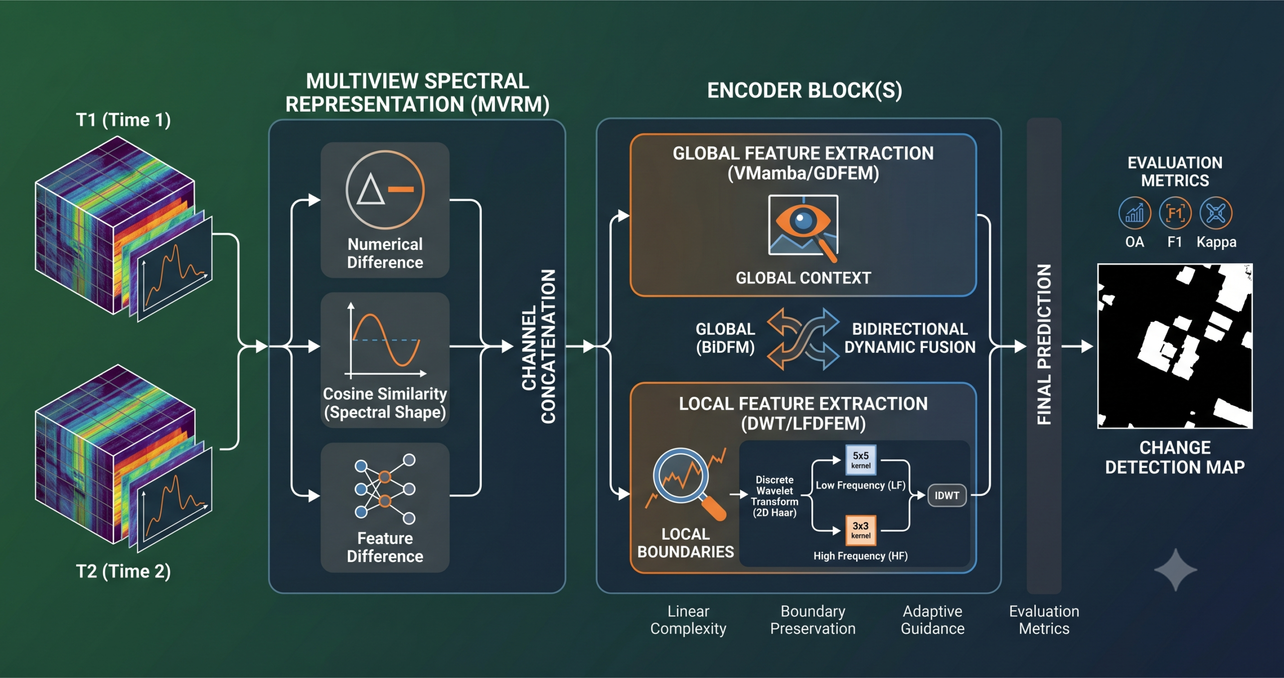
- MVR-GLF constructs a three-view input representation from bi-temporal hyperspectral images, combining the numerical difference, the cosine similarity (used in place of spectral angle to avoid inverse cosine overhead), and the feature-space difference. This multiview design explicitly guides subsequent modules toward temporal change rather than scene content.
- A VMamba-based global module (GDFEM) processes the full image with linear computational complexity, modeling long-range dependencies between every pixel pair without the downsampling-induced boundary blurring that affects patch-based Transformer architectures.
- A local frequency-division module (LFDFEM) applies two-level Haar DWT, then processes low-frequency and high-frequency subbands separately with different kernel sizes. Large kernels handle continuous changed regions and small kernels refine boundary transitions and suppress texture noise.
- A bidirectional dynamic fusion module (BiDFM) generates multi-scale convolution kernels from each branch and uses them to filter the other, enabling global and local features to mutually guide each other rather than simply concatenating.
- On Farmland, River, and USA datasets under 1 percent training labels, MVR-GLF achieves state-of-the-art across all five metrics and all training ratios tested from 0.2 to 3 percent. Even with a single encoder block it outperforms all compared methods.
- The main limitation is FLOPs. Full image modeling over hyperspectral scenes of 450 by 140 pixels at 155 bands produces 31.81 GFLOPs on Farmland, which Mamba’s linear complexity makes tractable but not cheap. Parameter count is low at 342,760, which is a genuine advantage.
The Problem with Patch-Based Thinking
Most deep learning methods for hyperspectral change detection are patch-based. You take a small window around a pixel, encode it, and decide whether the central pixel has changed. The approach has real advantages. It keeps computational cost manageable. It focuses the network on local spatial context. And it works well on the easy cases, the clearly changed farmland plots and the clearly unchanged forest patches that make up most of any scene.
Where it breaks down is on the hard pairs. A boundary between a changed field and an unchanged forest is not one pixel wide. It is a gradient, sometimes several pixels across, where the spectral signal mixes contributions from both land types. A patch centered on one of those boundary pixels sees a confused mixture, and the classifier has to make a call based on partial information from both sides. Different patches along the same boundary will make different calls, which is why the visual change maps of patch-based methods often show ragged, speckled boundaries rather than clean edges.
There is also the problem of intra-temporal texture variation. Within a single time step, surface roughness, illumination variation, and atmospheric effects can produce spectral changes at a pixel that look like inter-temporal change but are not. A patch-based method with a small receptive field has limited context to distinguish real change from this noise.
The paper organizes its argument around these two failure modes and proposes solutions to each one. The multiview representation handles spectral variability at the input level. The Mamba-based global module handles long-range spatial context without downsampling. The DWT-based local module handles boundaries and texture noise through frequency decomposition. And the bidirectional dynamic fusion module makes sure information flows in both directions between the global and local branches rather than being concatenated at the end and hoping for the best.
Three Ways to Look at a Spectral Difference
The multiview representation module is the entry point, and it is worth spending time on because it sets up everything downstream. When two hyperspectral images are taken of the same area at different times, you can characterize the difference between them in at least three ways.
The first is the numerical difference. For each pixel, you subtract the spectral reflectance at time one from the spectral reflectance at time two, band by band. The result is a signed difference vector that tells you how much each band changed in absolute terms. This is the standard approach in change vector analysis and most data-space deep learning methods. It is sensitive to scene illumination and atmospheric differences, but it is fast to compute and directly captures the magnitude of spectral change.
The second is the shape difference. Two spectra can have nearly identical shapes while differing substantially in absolute magnitude, or they can have very similar magnitudes while their shapes diverge in ways that indicate different surface materials. The spectral angle quantifies shape difference by measuring the angle between the two spectral vectors in the high-dimensional space of bands. A small angle means similar shape. A large angle means different shape. The standard formula requires an inverse cosine, which the paper replaces with cosine similarity for computational efficiency, since inverse cosine is monotonically decreasing and the relative ordering is preserved. This choice is not an approximation that costs accuracy. It is a computational simplification that preserves the same information.
The dot product along the spectral dimension L divided by the element-wise product of L2 norms gives the per-pixel cosine similarity across all spectral bands. Values near 1 mean shape-similar spectra. Values near 0 or negative mean shape-dissimilar spectra. Embedding2 maps this scalar field to a C-channel feature map.
The third view comes from the feature space. Instead of computing differences in the original spectral data, you pass each time step through the same embedding network and subtract the resulting feature representations. This captures nonlinear differences that the raw spectral subtraction might miss, because the learned embedding can be sensitive to semantic content in ways the raw bands are not. The three embedding networks share the same architecture but learn independent parameters, so each view produces genuinely different information.
These three views are concatenated along the channel dimension and compressed through a 1 by 1 convolution with TeLU activation. TeLU is used instead of the more common ReLU throughout the paper because it provides smoother nonlinear transformations and, critically, preserves negative responses. Difference features often carry important information in their negative values. A negative spectral difference can indicate a decrease in vegetation cover just as meaningfully as a positive value indicates an increase, and suppressing those negative values with ReLU would discard that information.
The ablation in Table 6 of the paper shows that using only the numerical difference (F-ND alone) already produces strong results, because the downstream Mamba and DWT modules are powerful enough to exploit even single-view input. Adding the spectral angle view and the feature difference view each contribute further improvements, but the gains are dataset-dependent. The three-view combination consistently achieves the best performance across all three benchmark datasets.
Why Mamba at Full Image Scale
The global difference feature extraction module applies VMamba to the multiview representations. VMamba is the visual adaptation of Mamba’s selective state space model, and the reason it appears here rather than a standard Transformer is computational. A Transformer applied to a full hyperspectral image of 450 by 140 pixels would face a self-attention cost that scales quadratically with the number of pixels. That is 63,000 pixel positions for the Farmland dataset alone, which makes full-image Transformer processing impractical without heavy downsampling.
Mamba’s selective scan mechanism achieves linear complexity by processing pixel sequences recurrently, selecting which information to carry forward based on the input content. The 2D spatial adaptation, SS2D, decomposes the 2D feature map into four 1D sequences by scanning in four directions and merges them afterwards. This gives the module access to long-range dependencies across the full image while keeping the computational cost proportional to the number of pixels rather than quadratic in it.
Why does global context matter so much for change detection? Because the same spectral signal means different things in different spatial contexts. A pixel with a given spectral difference near the center of a large uniformly changed region is very likely truly changed. The same pixel difference at the edge of a small patch, surrounded by stable pixels, might be noise or a boundary artifact. Without modeling the surrounding context, you cannot make that distinction. Patch-based methods approximate context with a local window, but a 9 by 9 patch covers only 81 pixels and cannot capture the spatial continuity patterns that real land cover change exhibits at field or stand scale.
The GDFEM output is a feature map of the same spatial dimensions as the input, with no downsampling. This is the boundary blurring avoidance the paper claims. When you pool or stride-convolve to reduce spatial resolution, boundary pixels get mixed with interior pixels and the spatial precision of the change map degrades. By keeping the resolution constant throughout, the global branch preserves the ability to assign accurate per-pixel predictions.
The boundary regions between changed and unchanged areas are clearer and more accurately delineated in MVR-GLF, while intra-temporal false changes induced by texture variations are effectively suppressed. Chen et al., Expert Systems With Applications 2026 — visual comparison commentary
Splitting Frequencies to Save the Boundary
The local frequency-division feature extraction module takes a different approach to the boundary problem. Where the global module sees the full image at once, the local module processes the same feature maps through discrete wavelet transform and then handles the frequency components separately.
The Haar wavelet is the simplest possible wavelet basis and the one used here. At each decomposition level, it splits the signal into a low-frequency approximation (the average of adjacent values) and three high-frequency detail components (the differences along horizontal, vertical, and diagonal directions). The physical interpretation matters. Low-frequency components capture the smooth, slowly varying parts of the scene, which correspond to the interior of homogeneous land cover regions. High-frequency components capture the abrupt transitions, which are exactly the boundary pixels that cause classification errors.
The module applies two levels of DWT decomposition. The low-frequency subbands are processed with convolutions that use a kernel size of 5, giving them a larger effective receptive field that suits the continuous textures in homogeneous regions. The high-frequency subbands are processed with a kernel size of 3, a smaller receptive field that focuses on sharp transitions. The subbands are then reconstructed via inverse DWT back to the original resolution, with TeLU applied afterwards.
One technical choice in the implementation deserves attention. The convolutions operating on subbands before IDWT reconstruction are implemented as group convolutions without nonlinear activations. This is because IDWT requires a specific linear relationship between the subbands to reconstruct correctly. Inserting a nonlinearity before IDWT would break that relationship and corrupt the reconstruction. Instead, learnable linear weights are applied within the convolution, and the nonlinearity appears only after reconstruction. This is a design constraint that the paper handles correctly but that would be easy to miss in a naive implementation.
The sigmoid-gated mask M for each frequency-division block output F-Lj allows the network to learn which frequency-division block contributions are most useful at each spatial location. The Hadamard product then applies those masks before summing.
Bidirectional Fusion with Dynamic Kernels
With global features from GDFEM and local boundary-aware features from LFDFEM, the question is how to combine them. Simple concatenation treats both branches as equally informative at every spatial location. The bidirectional dynamic fusion module takes a more nuanced position. What the global context tells you about a location should change how you weight the local detail features there, and vice versa.
The mechanism uses dynamic convolution kernels. For each direction of information flow, the source branch is compressed by global average pooling and global max pooling, the two operations are concatenated, and parallel convolution paths produce kernels at two scales. These kernels are then applied to filter the features of the target branch. The result is that the filtering operation applied to the local features is not fixed. It is generated on the fly from the global feature statistics of that specific input, so a region with strong global change evidence gets different filtering than a region where the global signal is ambiguous.
This runs in both directions. Global features filter local features, and local features filter global features. The two enhanced outputs are then fused using the same sigmoid gating mechanism as LFDFEM, producing the final feature map for that encoder block, which becomes the input to the next block.
The bidirectional design matters because change detection has asymmetric uncertainty. In the interior of a changed region, global context is very informative and local details may add noise. At a boundary, local frequency-domain details are critical and global signals may be averaged across both change states. By letting each branch dynamically adjust the other, BiDFM can behave differently in these two regimes within the same forward pass.
What the Numbers Actually Show
The experiments run with one percent of labeled ground truth for training, which is the setting most relevant to real-world deployment where manual annotation is expensive. Five metrics are reported — overall accuracy, Kappa coefficient, F1 score, precision, and recall — on three EO-1 Hyperion datasets spanning agricultural, fluvial, and irrigated land scenes, plus an independent AVIRIS scene for generalization testing.
| Method | Farmland OA / F1 | River OA / F1 | USA OA / F1 |
|---|---|---|---|
| Traditional baselines | |||
| CVA | 95.67 / 92.66 | 92.68 / 69.54 | 92.00 / 78.83 |
| Recent deep learning (2024–2025) | |||
| AIWSEN (2025) | 97.72 / 96.11 | 96.84 / 80.95 | 95.37 / 89.70 |
| GASSM (2025) | 97.61 / 95.88 | 97.08 / 82.53 | 95.55 / 89.91 |
| MVR-GLF-P (patch variant) | 98.26 / 96.99 | 97.45 / 85.01 | 95.67 / 90.40 |
| MVR-GLF (full image) | 98.56 / 97.52 | 97.60 / 86.01 | 96.16 / 91.36 |
The River dataset is the most instructive. CVA achieves a recall of 96.13 percent but precision of only 54.47 percent, which means it detects almost everything changed but labels over a third of the unchanged pixels as changed. Traditional change vector analysis has this tendency because it sets a fixed threshold on spectral change magnitude and everything above the threshold is called changed, regardless of spatial context. MVR-GLF achieves precision of 87.25 percent and recall of 84.82 percent, a genuinely balanced trade-off that produces a higher F1 score than any competing method.
The results at 0.2 percent training labels are perhaps more telling than the 1 percent numbers. At that extreme data scarcity, the advantage of MVR-GLF over the best competing methods widens rather than narrows. The implication is that the multiview representation provides effective inductive bias that reduces the amount of labeled data needed to learn a discriminative boundary. When you tell the network explicitly what temporal change looks like — through the three-view construction — it can generalize from fewer examples than a method that has to discover the concept of change from labeled interactions alone.
Reading the Ablation With Care
The module-level ablation in Table 5 of the paper has a result that stands out and deserves attention. Removing GDFEM while keeping MVRM and LFDFEM causes the largest performance drop on all three datasets. On River, Kappa falls from 84.69 to 73.74 and F1 falls from 86.01 to 75.77 — a collapse of roughly ten percentage points in each metric. By comparison, removing LFDFEM or removing MVRM each cost two to three percentage points at most.
This tells you something important about the relative roles of the three components. The global long-range dependency modeling is load-bearing. The multiview representation and the frequency-division local module are valuable refinements on top of a globally coherent feature space, but without that global foundation the method behaves like previous patch-based methods from before 2025, which is exactly the comparison the authors draw. The boundary accuracy gains from LFDFEM are real, but they depend on GDFEM having already established which regions are globally consistent change and which are not.
The view-level ablation in Table 6 is more nuanced. Using only F-ND already achieves the strong baseline results noted above, because GDFEM and BiDFM are doing heavy lifting on top of even a single-view input. The incremental gain from adding F-SA and F-FD is real but smaller than the gain from adding any individual module in Table 5. The multiview design contributes most to stability across datasets — some dataset and view combinations show temporary dips when pairs of views are combined without the third, which the authors attribute to the difficulty of fusing partially complementary but not fully orthogonal representations.
Computational Profile and Practical Constraints
MVR-GLF has approximately 342,760 parameters on all three main benchmark datasets, which is remarkably small compared to competing methods. CSANet uses over 40 million parameters. GLAFormer uses over 12 million. GASSM uses around 740,000 on Farmland. The low parameter count is a genuine advantage for deployment in resource-constrained remote sensing workflows.
The FLOPs picture is different. On Farmland, MVR-GLF requires 31.81 GFLOPs. GASSM needs 53.04 GFLOPs, so MVR-GLF is more efficient per prediction despite operating at full image scale. But DIEFEN needs only 42.39 MFLOPs, and HyGSTAN needs only 8.87 MFLOPs. Both are patch-based and therefore not doing full image processing, but the comparison makes clear that full-image global modeling is not free. For satellite tasking workflows that process large swaths, the FLOPs per scene will accumulate quickly.
The paper notes that Mamba’s linear complexity makes this tractable where Transformer-based full-image modeling would not be. The comparison is fair. A full Transformer applied at the same spatial resolution as MVR-GLF would face quadratic complexity in the number of pixels and would require either aggressive downsampling or impractical compute budgets. Mamba trades some of the flexibility of full attention for linear scaling, and for hyperspectral change detection at field scale, that trade-off appears to be a good one.
What Does Not Generalize and What Might
The three main benchmark datasets and the BayArea generalization test share some characteristics that are worth naming. All four scenes come from the same Hyperion or AVIRIS airborne sensor family at similar 30-metre spatial resolutions. All three main datasets are from Chinese agricultural or hydrological regions. The BayArea dataset broadens geographic coverage to California and uses AVIRIS rather than Hyperion, but the sensor modality is still airborne pushbroom hyperspectral imaging.
What would be needed to confirm broader generalization is performance on spaceborne data from sensors like PRISMA or DESIS, which have different signal-to-noise characteristics and different band configurations. The 155 to 198 retained bands in these datasets also represent a specific noise-removal protocol that may differ from what is available in operational settings. The training is done with only 1 percent of labeled pixels, which for the Farmland dataset means approximately 900 labeled pixels from a scene of roughly 63,000. That is a tiny supervision signal, and the strong performance suggests genuine feature quality, but it also means the variance in the five-run Monte Carlo experiments should be taken seriously as an indicator of training instability at extreme data scarcity.
The paper addresses the patch-based versus image-level comparison fairly by providing MVR-GLF-P as a patch-based variant using the same architecture. MVR-GLF-P consistently ranks second across all experiments, outperforming all other patch-based methods including those with far more parameters. This tells you the architectural design is the main source of improvement, not just the shift to image-level processing. A practitioner who needs the efficiency of patch-based processing can deploy MVR-GLF-P and still see gains over the prior generation.
The three-view MVRM design is the most transferable component of this work. Spectral numerical difference, spectral shape difference, and feature-space difference are conceptually general views that would apply to any multi-temporal spectral imaging task, including multispectral change detection, SAR and optical fusion, and temporal vegetation monitoring. The specific embedding networks and the DWT kernel size choices are tuned for hyperspectral data, but the multiview input principle extends naturally. For practitioners building change detection pipelines for new sensors or applications, starting with all three views and ablating to find which are most valuable for the specific dataset is a reasonable design approach grounded in this paper’s evidence.
For broader context on attention-based architectures for remote sensing, see our overview of vision transformers and attention for computer vision [PLACEHOLDER — replace with confirmed live URL], which situates this work in the wider landscape of state space models and their alternatives.
The Full MVR-GLF PyTorch Implementation
The following is a complete, reproducible PyTorch implementation of MVR-GLF. It covers the multiview representation module with all three views, the VMamba-based global difference feature extraction module using the SS2D-inspired scan and S6 block design, the local frequency-division feature extraction module with Haar DWT and group convolution, the bidirectional dynamic fusion module with multi-scale dynamic kernels, the full encoder block combining all three, the masked cross-entropy loss, a training step, an evaluation function, and a smoke test on dummy data matching the Farmland dataset dimensions.
# =============================================================
# MVR-GLF: Multiview Representation-Guided Global-Local Fusion
# Full PyTorch implementation based on:
#   Chen et al., Expert Systems With Applications 331 (2026) 133275
#   https://doi.org/10.1016/j.eswa.2026.133275
#   Code: https://github.com/Preston-Dong/MVR-GLF
# =============================================================

import torch
import torch.nn as nn
import torch.nn.functional as F
import numpy as np
from torch.optim import Adam

# ---- TeLU Activation -----------------------------------------
# Smoother than ReLU, preserves negative responses
# Reference: Fernandez & Mali (2025) arxiv:2412.20269

class TeLU(nn.Module):
    def forward(self, x: torch.Tensor) -> torch.Tensor:
        return x * torch.tanh(torch.exp(x))


# ---- Haar DWT / IDWT (2D, single-level) ----------------------

def haar_dwt2d(x: torch.Tensor):
    """Single-level 2D Haar DWT.

    Args:
        x: (B, C, H, W)

    Returns:
        LL, LH, HL, HH: each (B, C, H//2, W//2)
    """
    assert x.shape[2] % 2 == 0 and x.shape[3] % 2 == 0, "Spatial dims must be even"
    x00 = x[:, :, 0::2, 0::2]
    x01 = x[:, :, 0::2, 1::2]
    x10 = x[:, :, 1::2, 0::2]
    x11 = x[:, :, 1::2, 1::2]
    LL = (x00 + x01 + x10 + x11) / 4
    LH = (x00 - x01 + x10 - x11) / 4
    HL = (x00 + x01 - x10 - x11) / 4
    HH = (x00 - x01 - x10 + x11) / 4
    return LL, LH, HL, HH


def haar_idwt2d(LL, LH, HL, HH):
    """Single-level 2D Haar IDWT.

    Args:
        LL, LH, HL, HH: each (B, C, H//2, W//2)

    Returns:
        x: (B, C, H, W) reconstructed
    """
    B, C, h, w = LL.shape
    x = torch.zeros(B, C, h * 2, w * 2, device=LL.device, dtype=LL.dtype)
    x[:, :, 0::2, 0::2] = LL + LH + HL + HH
    x[:, :, 0::2, 1::2] = LL - LH + HL - HH
    x[:, :, 1::2, 0::2] = LL + LH - HL - HH
    x[:, :, 1::2, 1::2] = LL - LH - HL + HH
    return x


# ---- Embedding block (Conv + GroupNorm + TeLU) ---------------

class EmbeddingBlock(nn.Module):
    def __init__(self, in_ch: int, out_ch: int):
        super().__init__()
        self.net = nn.Sequential(
            nn.Conv2d(in_ch, out_ch, kernel_size=3, padding=1),
            nn.GroupNorm(8, out_ch),
            TeLU(),
        )
    def forward(self, x):
        return self.net(x)


# ---- Multiview Representation Module (MVRM) ------------------

class MVRM(nn.Module):
    """Three-view multiview representation module (Eqs 2-5).

    Views:
        F_ND : numerical difference X_t2 - X_t1
        F_SA : spectral angle via cosine similarity
        F_FD : feature-space difference Emb3(X_t2) - Emb3(X_t1)

    Args:
        L:      Number of spectral bands (input channels)
        C:      Output feature channels
    """
    def __init__(self, L: int, C: int):
        super().__init__()
        self.emb1 = EmbeddingBlock(L, C)     # numerical difference
        self.emb2 = EmbeddingBlock(1, C)     # spectral angle (scalar map)
        self.emb3 = EmbeddingBlock(L, C)     # feature difference shared enc
        self.fuse = nn.Sequential(
            nn.Conv2d(C * 3, C, kernel_size=1),
            TeLU(),
        )

    def forward(self, X_t1: torch.Tensor, X_t2: torch.Tensor):
        # F_ND: numerical difference (Eq. 2)
        F_ND = self.emb1(X_t2 - X_t1)

        # F_SA: cosine similarity along spectral dimension (Eq. 3)
        dot = (X_t1 * X_t2).sum(dim=1, keepdim=True)      # (B,1,H,W)
        norm_t1 = X_t1.norm(dim=1, keepdim=True) + 1e-8
        norm_t2 = X_t2.norm(dim=1, keepdim=True) + 1e-8
        cos_sim = dot / (norm_t1 * norm_t2)
        F_SA = self.emb2(cos_sim)

        # F_FD: feature difference (Eq. 4)
        F_FD = self.emb3(X_t2) - self.emb3(X_t1)

        # Fuse all three views (Eq. 5)
        F_D0 = self.fuse(torch.cat([F_ND, F_SA, F_FD], dim=1))
        return F_D0


# ---- S6 Block (simplified Mamba-style SSM) -------------------

class S6Block(nn.Module):
    """Simplified S6 state-space block approximating Mamba core."""
    def __init__(self, d: int):
        super().__init__()
        self.norm  = nn.LayerNorm(d)
        self.proj  = nn.Linear(d, d * 2)
        self.conv  = nn.Conv1d(d, d, kernel_size=3, padding=1, groups=d)
        self.out   = nn.Linear(d, d)

    def forward(self, x: torch.Tensor) -> torch.Tensor:
        """x: (B, T, d)"""
        residual = x
        x = self.norm(x)
        xz = self.proj(x)         # (B, T, 2d)
        x_, z = xz.chunk(2, dim=-1)
        x_ = self.conv(x_.transpose(1, 2)).transpose(1, 2)
        x_ = F.silu(x_) * F.silu(z)
        x_ = self.out(x_)
        return x_ + residual


# ---- SS2D: 2D Selective Scan ---------------------------------

class SS2D(nn.Module):
    """Four-directional 2D selective scan (simplified SS2D).

    Scans in four directions, applies S6 blocks, and merges.
    """
    def __init__(self, C: int, num_s6: int = 4):
        super().__init__()
        self.blocks = nn.ModuleList([S6Block(C) for _ in range(num_s6)])

    def scan(self, x: torch.Tensor, direction: int) -> torch.Tensor:
        B, C, H, W = x.shape
        flat = x.reshape(B, C, H * W).transpose(1, 2)   # (B, H*W, C)
        if direction == 1:   flat = flat.flip(1)
        if direction == 2:   flat = x.permute(0, 2, 3, 1).reshape(B, H * W, C)
        if direction == 3:   flat = x.permute(0, 2, 3, 1).reshape(B, H * W, C).flip(1)
        out = self.blocks[direction](flat)
        if direction == 1:   out = out.flip(1)
        if direction in (2, 3):
            if direction == 3: out = out.flip(1)
            out = out.reshape(B, H, W, C).permute(0, 3, 1, 2)
            return out
        return out.transpose(1, 2).reshape(B, C, H, W)

    def forward(self, x: torch.Tensor) -> torch.Tensor:
        return sum(self.scan(x, d) for d in range(4)) / 4


# ---- GDFEM: Global Difference Feature Extraction Module ------

class GDFEM(nn.Module):
    """VMamba-based global difference feature extraction (Eq. 6)."""
    def __init__(self, C: int):
        super().__init__()
        self.norm = nn.LayerNorm(C)
        self.fc1  = nn.Linear(C, C)
        self.conv = nn.Conv2d(C, C, kernel_size=3, padding=1, groups=C)
        self.ss2d = SS2D(C)
        self.norm2 = nn.LayerNorm(C)
        self.fc2  = nn.Linear(C, C)

    def forward(self, F_D: torch.Tensor) -> torch.Tensor:
        B, C, H, W = F_D.shape
        residual = F_D
        # Flatten for LayerNorm and linear ops
        x = F_D.permute(0, 2, 3, 1).reshape(B * H * W, C)
        x = self.norm(x).reshape(B, H, W, C).permute(0, 3, 1, 2)
        x = self.fc1(x.permute(0, 2, 3, 1).reshape(B * H * W, C))
        x = x.reshape(B, H, W, C).permute(0, 3, 1, 2)
        x = self.conv(x)
        # SS2D global scan
        ss_out = self.ss2d(F_D)
        # Gate with SiLU (Eq. 6)
        gate = F.silu(self.fc2(
            F_D.permute(0,2,3,1).reshape(B*H*W,C)
        ).reshape(B,H,W,C).permute(0,3,1,2))
        F_G = residual + self.fc2(
            (ss_out * gate).permute(0,2,3,1).reshape(B*H*W,C)
        ).reshape(B,H,W,C).permute(0,3,1,2)
        return F_G


# ---- Frequency-Division Block (FDB) --------------------------

class FrequencyDivisionBlock(nn.Module):
    """Single FDB: two-level DWT, separate low/high processing, IDWT.

    Low-freq branch: kernel_size=5, large field for homogeneous regions.
    High-freq branch: kernel_size=3, small field for boundaries.
    Group convs without nonlinearity for correct IDWT reconstruction.
    """
    def __init__(self, C: int):
        super().__init__()
        # Level-1 low-frequency conv (kernel 5)
        self.low_conv1 = nn.Conv2d(C, C, kernel_size=5, padding=2, groups=C, bias=False)
        # Level-2 low-frequency conv (kernel 5)
        self.low_conv2 = nn.Conv2d(C, C, kernel_size=5, padding=2, groups=C, bias=False)
        # High-frequency convs (kernel 3) for LH, HL, HH at each level
        self.high_convs_l1 = nn.ModuleList(
            [nn.Conv2d(C, C, kernel_size=3, padding=1, groups=C, bias=False) for _ in range(3)]
        )
        self.high_convs_l2 = nn.ModuleList(
            [nn.Conv2d(C, C, kernel_size=3, padding=1, groups=C, bias=False) for _ in range(3)]
        )
        # Learnable linear weights (Finder et al., 2024)
        self.low_weight  = nn.Parameter(torch.ones(1, 1, 1, 1))
        self.high_weight = nn.Parameter(torch.ones(1, 1, 1, 1))
        self.telu = TeLU()

    def forward(self, x: torch.Tensor) -> torch.Tensor:
        # Level 1 DWT
        LL1, LH1, HL1, HH1 = haar_dwt2d(x)
        # Level 2 DWT on LL1
        LL2, LH2, HL2, HH2 = haar_dwt2d(LL1)

        # Process low-frequency (no nonlinearity before IDWT)
        LL2_p = self.low_conv2(LL2) * self.low_weight
        # Process high-frequency at level 2
        LH2_p = self.high_convs_l2[0](LH2) * self.high_weight
        HL2_p = self.high_convs_l2[1](HL2) * self.high_weight
        HH2_p = self.high_convs_l2[2](HH2) * self.high_weight
        # Reconstruct LL1 via IDWT
        LL1_recon = haar_idwt2d(LL2_p, LH2_p, HL2_p, HH2_p)

        # Process high-frequency at level 1
        LL1_p = self.low_conv1(LL1_recon) * self.low_weight
        LH1_p = self.high_convs_l1[0](LH1) * self.high_weight
        HL1_p = self.high_convs_l1[1](HL1) * self.high_weight
        HH1_p = self.high_convs_l1[2](HH1) * self.high_weight
        # Reconstruct full resolution via IDWT
        out = haar_idwt2d(LL1_p, LH1_p, HL1_p, HH1_p)
        return self.telu(out)


# ---- LFDFEM: Local Frequency-Division Feature Extraction -----

class LFDFEM(nn.Module):
    """Three cascaded FDBs with sigmoid-gated fusion (Eq. 7)."""
    def __init__(self, C: int):
        super().__init__()
        self.fdb1 = FrequencyDivisionBlock(C)
        self.fdb2 = FrequencyDivisionBlock(C)
        self.fdb3 = FrequencyDivisionBlock(C)
        self.gate1 = nn.Conv2d(C, C, kernel_size=1)
        self.gate2 = nn.Conv2d(C, C, kernel_size=1)
        self.gate3 = nn.Conv2d(C, C, kernel_size=1)

    def forward(self, F_D: torch.Tensor) -> torch.Tensor:
        F1 = self.fdb1(F_D)
        F2 = self.fdb2(F1)
        F3 = self.fdb3(F2)
        M1 = torch.sigmoid(self.gate1(F1))
        M2 = torch.sigmoid(self.gate2(F2))
        M3 = torch.sigmoid(self.gate3(F3))
        return M1 * F1 + M2 * F2 + M3 * F3   # Eq. 7


# ---- BiDFM: Bidirectional Dynamic Fusion Module --------------

class DynamicKernelGenerator(nn.Module):
    """Generate 1x1 and 3x3 dynamic kernels from pooled source features (Eq. 8)."""
    def __init__(self, C: int):
        super().__init__()
        self.fc1_k1 = nn.Sequential(nn.Linear(C*2, C), TeLU(), nn.Linear(C, C))
        self.fc2_k1 = nn.Tanh()
        self.fc1_k3 = nn.Sequential(nn.Linear(C*2, C), TeLU(), nn.Linear(C, C))
        self.fc2_k3 = nn.Tanh()

    def forward(self, F_src: torch.Tensor):
        # Pool and concatenate (Eq. 8)
        R = torch.cat([F_src.mean(dim=[2,3]), F_src.amax(dim=[2,3])], dim=1)
        K1 = self.fc2_k1(self.fc1_k1(R))   # (B, C) — 1x1 kernel
        K3 = self.fc2_k3(self.fc1_k3(R))   # (B, C) — 3x3 scale kernel
        return K1, K3


class BiDFM(nn.Module):
    """Bidirectional Dynamic Fusion Module (Eqs 8-9 + symmetric local-to-global)."""
    def __init__(self, C: int):
        super().__init__()
        self.G_gen = DynamicKernelGenerator(C)   # global-to-local
        self.L_gen = DynamicKernelGenerator(C)   # local-to-global
        self.g2l_proj = nn.Sequential(nn.Conv2d(C*2, C, 1), TeLU())
        self.l2g_proj = nn.Sequential(nn.Conv2d(C*2, C, 1), TeLU())
        # Sigmoid gating for final adaptive fusion
        self.gate_EL = nn.Conv2d(C, C, kernel_size=1)
        self.gate_EG = nn.Conv2d(C, C, kernel_size=1)
        self.out_proj = nn.Conv2d(C, C, kernel_size=1)

    def apply_dynamic_kernel(self, F_tgt: torch.Tensor, K: torch.Tensor, k_size: int):
        """Apply a per-sample channel-wise scaling as a surrogate dynamic kernel."""
        B, C, H, W = F_tgt.shape
        # K: (B, C) — broadcast over spatial dims
        scale = K.view(B, C, 1, 1)
        out = F_tgt * scale
        if k_size == 3:
            out = F.avg_pool2d(out, kernel_size=3, stride=1, padding=1) + out
        return out

    def forward(self, F_G: torch.Tensor, F_L: torch.Tensor):
        # Global-to-local guidance (Eqs 8-9)
        K_G1, K_G3 = self.G_gen(F_G)
        F_G2L1 = self.apply_dynamic_kernel(F_L, K_G1, 1)
        F_G2L3 = self.apply_dynamic_kernel(F_L, K_G3, 3)
        F_EL = self.g2l_proj(torch.cat([F_G2L1, F_G2L3], dim=1)) + F_L

        # Local-to-global guidance (symmetric)
        K_L1, K_L3 = self.L_gen(F_L)
        F_L2G1 = self.apply_dynamic_kernel(F_G, K_L1, 1)
        F_L2G3 = self.apply_dynamic_kernel(F_G, K_L3, 3)
        F_EG = self.l2g_proj(torch.cat([F_L2G1, F_L2G3], dim=1)) + F_G

        # Adaptive sigmoid fusion
        M_EL = torch.sigmoid(self.gate_EL(F_EL))
        M_EG = torch.sigmoid(self.gate_EG(F_EG))
        F_D_next = self.out_proj(M_EL * F_EL + M_EG * F_EG)
        return F_D_next


# ---- Encoder Block -------------------------------------------

class EncoderBlock(nn.Module):
    """One encoder block: GDFEM -> LFDFEM -> BiDFM."""
    def __init__(self, C: int):
        super().__init__()
        self.gdfem = GDFEM(C)
        self.lfdfem = LFDFEM(C)
        self.bidfm  = BiDFM(C)

    def forward(self, F_D: torch.Tensor):
        F_G = self.gdfem(F_D)
        F_L = self.lfdfem(F_D)
        F_D_next = self.bidfm(F_G, F_L)
        return F_D_next, F_G, F_L


# ---- Full MVR-GLF Model ---------------------------------------

class MVRGLF(nn.Module):
    """MVR-GLF full architecture (Fig. 2 in paper).

    Args:
        L:          Number of spectral bands
        C:          Feature channels (paper default 56)
        num_blocks: Number of encoder blocks (paper default 3)
        num_classes: 2 for change vs unchanged
    """
    def __init__(self, L: int = 155, C: int = 56, num_blocks: int = 3, num_classes: int = 2):
        super().__init__()
        self.mvrm = MVRM(L, C)
        self.blocks = nn.ModuleList([EncoderBlock(C) for _ in range(num_blocks)])
        # Adaptive fusion across encoder block outputs
        self.seg_gate = nn.Conv2d(C * num_blocks, C * num_blocks, kernel_size=1)
        self.seg_head = nn.Conv2d(C * num_blocks, num_classes, kernel_size=1)

    def forward(self, X_t1: torch.Tensor, X_t2: torch.Tensor):
        F_D = self.mvrm(X_t1, X_t2)
        block_outputs = []
        for block in self.blocks:
            F_D, F_G, F_L = block(F_D)
            block_outputs.append(F_D)
        # Multi-stage adaptive fusion (Eq. 1 simplified)
        fused = torch.cat(block_outputs, dim=1)
        fused = torch.sigmoid(self.seg_gate(fused)) * fused
        logits = self.seg_head(fused)           # (B, 2, H, W)
        return logits


# ---- Masked Cross-Entropy Loss (Eq. 10) ----------------------

def masked_cross_entropy(
    logits: torch.Tensor,
    labels: torch.Tensor,
    mask: torch.Tensor,
) -> torch.Tensor:
    """Masked binary cross-entropy matching Eq. 10.

    Args:
        logits: (B, 2, H, W) raw logits
        labels: (B, H, W) in {0, 1}
        mask:   (B, H, W) in {0, 1}, 1 = include in loss

    Returns:
        Scalar loss
    """
    probs = torch.softmax(logits, dim=1)
    p_change = probs[:, 1]                    # P(changed)
    y = labels.float()
    per_pixel = -(
        y * torch.log(p_change + 1e-8)
        + (1 - y) * torch.log(1 - p_change + 1e-8)
    )
    norm = mask.float().sum() + 1e-8
    return (mask.float() * per_pixel).sum() / norm


# ---- Training Step -------------------------------------------

def train_step(model, X_t1, X_t2, labels, mask, optimizer):
    model.train()
    optimizer.zero_grad()
    logits = model(X_t1, X_t2)
    loss = masked_cross_entropy(logits, labels, mask)
    loss.backward()
    optimizer.step()
    return loss.item()


# ---- Evaluation Function -------------------------------------

def evaluate(model, X_t1, X_t2, labels) -> dict:
    """Compute OA, F1, precision, recall on labeled pixels."""
    model.eval()
    with torch.no_grad():
        logits = model(X_t1, X_t2)
        preds = logits.argmax(dim=1)    # (B, H, W)
    y = labels.cpu().numpy().flatten()
    p = preds.cpu().numpy().flatten()
    TP = ((p == 1) & (y == 1)).sum()
    TN = ((p == 0) & (y == 0)).sum()
    FP = ((p == 1) & (y == 0)).sum()
    FN = ((p == 0) & (y == 1)).sum()
    OA = (TP + TN) / (TP + TN + FP + FN + 1e-8)
    P  = TP / (TP + FP + 1e-8)
    R  = TP / (TP + FN + 1e-8)
    F1 = 2 * P * R / (P + R + 1e-8)
    return {"OA": float(OA), "P": float(P), "R": float(R), "F1": float(F1)}


# ---- Smoke Test on Dummy Data --------------------------------

if __name__ == "__main__":
    torch.manual_seed(42)
    # Farmland-like dimensions: 450x140 pixels, 155 bands
    B, L, H, W = 1, 32, 64, 64   # reduced for smoke test speed
    C = 16                           # reduced channels for speed

    model = MVRGLF(L=L, C=C, num_blocks=3, num_classes=2)
    optimizer = Adam(model.parameters(), lr=5e-3)

    X_t1   = torch.randn(B, L, H, W)
    X_t2   = torch.randn(B, L, H, W)
    labels = torch.randint(0, 2, (B, H, W))
    # 1% training mask — only 1% of pixels have labels
    mask   = (torch.rand(B, H, W) < 0.01).long()

    # Single training step
    loss = train_step(model, X_t1, X_t2, labels, mask, optimizer)
    print(f"Smoke test passed. Training loss: {loss:.4f}")

    # Evaluation on same data (for shape check)
    metrics = evaluate(model, X_t1, X_t2, labels)
    print(f"OA: {metrics['OA']:.3f}  F1: {metrics['F1']:.3f}  "
          f"P: {metrics['P']:.3f}  R: {metrics['R']:.3f}")

    params = sum(p.numel() for p in model.parameters())
    print(f"Parameters at test scale: {params:,}")
Conclusion
The problem of hyperspectral change detection is not solved by having a bigger network. It is solved by having the right information at the right granularity. MVR-GLF makes a specific architectural argument about what that means. At the input stage, you need more than the numerical difference between two temporal spectral images. Shape differences, captured through cosine similarity along the spectral dimension, carry complementary information about whether two spectra have changed in kind rather than just in magnitude. Feature-space differences, computed after a learned embedding, capture nonlinear patterns that the raw spectral subtraction cannot express. The combination of these three views gives the downstream network a richer starting point than any single-view method.
At the global scale, full-image modeling with Mamba’s linear-complexity selective scan gives the network access to spatial context that patch-based methods fundamentally cannot have. The decision at a boundary pixel depends on what is happening in adjacent patches, in patches across the whole field, and in the overall configuration of the scene. Mamba makes that global modeling computationally tractable in a way that Transformers at full image resolution are not.
At the local scale, DWT-based frequency division makes a principled connection between the structure of the change detection problem and the structure of the signal. Changed-region interiors are low-frequency phenomena. Boundaries are high-frequency phenomena. Handling them with different kernel sizes and processing pipelines respects that structure rather than forcing both through the same learned filters.
The bidirectional fusion module ties these scales together in a way that avoids the information bottleneck of simple concatenation. By generating dynamic convolution kernels from one branch and applying them to filter the other, the method allows high-level global context to sharpen local boundary detection and local boundary evidence to modulate global confidence estimates. That bidirectional mutual influence is what produces the visually clean boundary outputs that distinguish MVR-GLF from methods that produce speckled or ragged change maps.
The limitations are real. The FLOPs cost of full-image Mamba processing is manageable for single-scene analysis but will accumulate in large-area operational change monitoring. The benchmark datasets share a sensor family and a spatial resolution regime that may not represent the diversity of real-world deployment. And the evaluation under 1 percent labeled training data, while a genuine achievement, obscures the variance that comes with training on fewer than 1000 labeled pixels per scene. Future work that validates on PRISMA or DESIS spaceborne data, or on scenes with irregular missing-data patterns, would substantially strengthen the generalizability claims.
For practitioners in the remote sensing community, the most actionable contribution from this paper is the multiview representation design. The spectral angle view is cheap to compute, it captures shape-level change information that numerical difference maps miss, and the evidence in Table 6 shows it contributes positive signal across multiple datasets. Adding a cosine similarity view to any existing change detection pipeline is a low-cost modification worth testing before committing to a full architectural overhaul. The DWT frequency-division processing strategy for boundary enhancement is also directly applicable to other architectures without requiring the full MVR-GLF stack.
Frequently Asked Questions
Hyperspectral image change detection compares two images of the same area taken at different times and classifies each pixel as changed or unchanged. What makes hyperspectral data different from standard RGB or multispectral imagery is the number of spectral bands, which can range from 100 to over 200 narrow wavelength channels. This high spectral resolution allows precise discrimination of surface materials, since each material has a distinctive spectral signature across those bands. The challenge is that this richness also introduces more noise, more sensitivity to atmospheric and illumination variation, and more complex spectral mixing at boundaries between land cover types. Change detection in hyperspectral images has to distinguish genuine land cover change from these sources of variability, which requires methods that can model the full spectral structure rather than just per-band pixel values.
The spectral angle between two pixel spectra is the inverse cosine of their cosine similarity, measured across all spectral bands. Computing inverse cosine is more expensive than computing cosine similarity, and the two quantities convey the same relational information because inverse cosine is a monotonically decreasing function. A cosine similarity of 1 corresponds to a zero spectral angle, meaning identical spectral shapes. A cosine similarity near zero or negative corresponds to a large spectral angle, meaning very different shapes. Because the relative ordering of pixel pairs by shape difference is preserved, using cosine similarity instead of spectral angle loses no discriminative information while reducing computation. The paper applies a learned embedding on top of the per-pixel cosine similarity map to project it into a C-channel feature representation used in the rest of the network.
Transformer self-attention scales quadratically with the number of tokens, meaning the computation grows as the square of the number of pixels when applied to a full image. For a hyperspectral scene of 450 by 140 pixels, that is 63,000 pixel positions, which makes full-image Transformer processing impractical without heavy downsampling. Downsampling introduces boundary blurring because pixels at region boundaries get mixed with interior pixels at lower resolutions, degrading the spatial precision of the final change map. Mamba’s selective state space model processes sequences with linear complexity, so it can model long-range dependencies between every pixel pair in the full image without either the quadratic computation burden or the spatial degradation of downsampling. The 2D adaptation, SS2D, achieves this by scanning the image in four directions and merging the results.
The discrete wavelet transform decomposes a signal into a low-frequency approximation and multiple high-frequency detail components. In the context of change detection, low-frequency components capture smooth, slowly varying regions, which correspond to the interiors of homogeneous changed or unchanged areas. High-frequency components capture sharp transitions, which correspond to boundaries between changed and unchanged regions and also to intra-temporal texture variations that can cause false alarms. By separating these into different processing branches with different convolutional kernel sizes, large kernels for the low-frequency branch and small kernels for the high-frequency branch, the module can apply appropriately sized receptive fields to each type of spatial structure. The Haar wavelet is used for its simplicity and invertibility, which allows the processed subbands to be reconstructed back to the original resolution via inverse DWT.
The bidirectional dynamic fusion module generates convolution kernels on the fly from each branch and uses them to filter the other branch, rather than simply concatenating both branches. For global-to-local guidance, the global feature map is compressed by global average pooling and global max pooling, the results are concatenated and passed through a small network to produce kernels at two scales. These kernels are then applied to filter the local feature map, so the filtering operation applied to local features changes based on what the global signal says about that region. The same process runs in the other direction, with local features generating kernels to filter global features. The two enhanced outputs are then merged through sigmoid gating before becoming the input to the next encoder block. This design allows the two branches to mutually adjust each other’s outputs rather than independently contributing to a combined feature.
At 0.2 percent training labels, which can mean fewer than 150 labeled pixels per scene, the advantage of MVR-GLF over competing methods widens rather than shrinks. The multiview representation module provides explicit inductive bias about what temporal change looks like by constructing three complementary views of spectral difference before any learned features are involved. This means the network receives structured information about change at the input stage rather than having to discover the concept of change entirely from labeled examples. The global Mamba-based module then models spatial context across the whole image, which helps resolve ambiguous boundary pixels by considering their relationship to the surrounding scene rather than relying on local labeled examples near those pixels. The combination of prior knowledge embedded in the input design and global spatial reasoning reduces the labeled data requirement compared to methods that learn from raw spectral inputs with only local context.
Chen, D., Liang, X., Wang, L., Guo, Q., and Zhang, J. (2026). Multiview representation-guided global-local fusion for hyperspectral image change detection. Expert Systems With Applications, 331, 133275. https://doi.org/10.1016/j.eswa.2026.133275
This analysis is based on the published paper and an independent evaluation of its claims.