Imagine a user on a movie platform who rates each film across five dimensions: acting, directing, story, visuals, and an overall score. The platform knows, with fine-grained detail, not just what the person liked but why, across every film they have ever seen. That is genuinely useful for recommendations. It is also a privacy exposure most users have not thought about. A team from three Turkish universities decided to ask what happens when you apply formal local differential privacy to a system like this, and whether the answer is even tractable.
Key Points
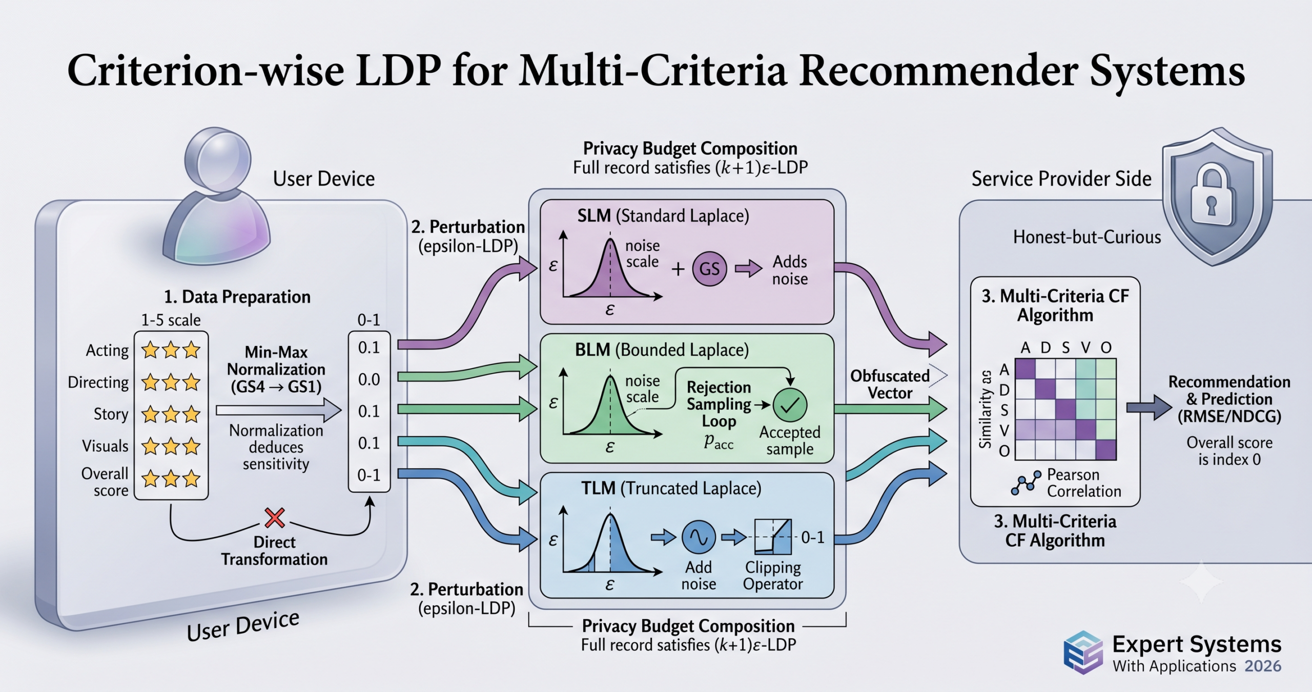
- This is the first published work to apply differential privacy within a multi-criteria collaborative filtering (MCCF) framework, addressing a gap that prior work had identified but left open.
- The framework perturbs each criterion independently using one of three Laplace mechanisms: Standard (SLM), Bounded (BLM), or Truncated (TLM), each of which produces a different tradeoff between noise control and computational cost.
- Because the mechanisms are applied per-criterion, each dimension satisfies epsilon-LDP individually. The full multi-criteria record satisfies a composed budget of (k plus 1) times epsilon, where k is the number of sub-criteria.
- BLM and TLM consistently outperform SLM under tight privacy budgets because they prevent noise from pushing ratings outside the valid rating range. SLM’s unbounded noise causes larger prediction errors when epsilon is small.
- Normalizing ratings to the zero-to-one interval before adding noise reduces the global sensitivity from 4 to 1, cutting noise magnitude by a factor of 4 for the same epsilon. This helps accuracy substantially at mid-range privacy settings.
- The optimal privacy budget appears around epsilon equal to ln(3) for YM20 and around ln(2) for YM10, both confirmed by RMSE analysis at the 95% confidence level.
Why Multi-Criteria Ratings Change the Privacy Calculus
Standard single-criterion recommender systems collect one number per user-item pair. Multi-criteria systems collect several. For Yahoo!Movies, the dataset used in this paper, that means acting, directing, storyline, visual appeal, and an overall grade per movie, all from the same user. The privacy exposure is not just larger in quantity. It is structurally different.
Yargic and Bilge (2017), cited in the paper’s background, showed that multi-criteria datasets carry unique privacy risks beyond those of single-criterion systems. Knowing not just that a user rated a film poorly, but that they rated the acting a 4 and the story a 1, reveals something about their aesthetic judgments that a simple overall score does not. These finer signals can be used to re-identify users, infer personality traits, or reconstruct private viewing histories with higher accuracy than overall ratings alone would permit.
Previous attempts at privacy-preserving MCCF are thin on the ground. The only prior work the authors identify is Yargic and Bilge (2019), which used a Randomized Perturbation Technique (RPT) to disguise multi-criteria ratings. RPT adds noise to data but provides no formal mathematical guarantees on how much information leaks. Differential privacy is different. It gives a quantitative bound on the privacy loss through the epsilon parameter, and that bound holds regardless of what background knowledge an adversary possesses.
The question the researchers at Eskisehir Technical University, Gümüshane University, and Bilecik Seyh Edebali University set out to answer is whether you can bring those formal guarantees into the MCCF setting without the multi-dimensional structure falling apart in the process.
The Three Mechanisms and What Separates Them
All three mechanisms share the same basic structure. You take a true rating, draw noise from a Laplace distribution whose scale is set to the global sensitivity divided by epsilon, and add the noise to the rating. The global sensitivity is just the width of the rating range, which for the one-to-five scale used in Yahoo!Movies is 4. The question is what happens when the noisy result falls outside the valid range.
SLM does nothing. The output can be any real number, including values far below 1 or far above 5. This is mathematically clean and easy to analyze. It is also the weakest performer when epsilon is small, because large noise samples frequently produce out-of-range values that are treated as legitimate perturbed ratings by the similarity computation on the service provider side. Those values distort user profiles in ways that are hard to recover from during prediction.
BLM uses rejection sampling. It draws from the same Laplace distribution but only accepts the sample if it falls within the valid range. It repeats until it gets an acceptable value. The resulting distribution is a Laplace restricted to the interval, properly normalized. This means the output is always a valid rating. The cost is computational. Under strict privacy settings, most samples are rejected before one is accepted, and the expected number of draws grows as epsilon shrinks. The paper reports that BLM’s disguising time on the YM10 dataset at epsilon equal to 0.1 is about 52.6 seconds, versus 13 seconds for SLM under the same conditions. That is a real operational cost.
TLM is the pragmatic middle ground. It draws Laplace noise and adds it to the rating, then clips the result to the valid range using a simple min-max operation. Any perturbed value below the lower bound becomes the lower bound. Any value above the upper bound becomes the upper bound. This is fast, always produces valid outputs, and avoids the rejection sampling overhead. The tradeoff is that clipping concentrates a disproportionate fraction of output values at the boundary points, which can introduce its own bias when the data distribution is already skewed toward extreme ratings.
That last point turns out to matter in practice. The Yahoo!Movies datasets used in this paper have a distribution heavily skewed toward ratings of 4 and 5. TLM’s clipping procedure piles even more probability mass at the upper boundary, which slightly inflates RMSE compared to BLM when epsilon is moderate. You can see the effect clearly in the paper’s figures, where BLM and TLM cross over around epsilon equal to ln(3) on the YM20 dataset.
The global sensitivity is the same for every criterion because each lives on the same rating scale. This is what makes the criterion-wise extension tractable. A single GS value of 4 (or 1 after normalization) applies across all five rating dimensions, which means the noise calibration is identical for each one. The paper frames this as a design choice rather than a convenience: equal sensitivity treatment ensures that no single criterion receives weaker privacy protection than another.
The Normalization Trick That Cuts Noise by a Factor of Four
Here is a detail that deserves more attention than papers of this type usually give it. The global sensitivity of an identity query on a one-to-five scale is simply five minus one, which is 4. The scale of the Laplace noise is then 4 divided by epsilon. At epsilon equal to 1, that is a noise scale of 4, which is enormous relative to a rating scale that only spans 4 units total. You are adding noise whose standard deviation is roughly equal to the full dynamic range of the variable you are trying to protect.
If you first rescale all ratings to lie between 0 and 1 using min max normalization, the global sensitivity drops to 1. The noise scale becomes 1 divided by epsilon. At epsilon equal to 1, that is a noise scale of 1 rather than 4. Every noise sample is four times smaller for the same epsilon value. You get the same formal privacy guarantee with a fraction of the perturbation.
The paper calls the unnormalized version DP based MCCF with GS equal to 4, and the normalized version with GS equal to 1. The normalized version consistently achieves lower RMSE and MAE at the same epsilon, with the benefit most visible at smaller epsilon values where noise is largest. The effect is modest for BLM at larger epsilon values, where the noise is already small enough to stay within the rating range even without normalization. But at epsilon equal to 0.1, the normalized SLM drops RMSE from 2.3705 to 2.3759 on YM20. That is a small absolute difference, but it is statistically significant at the 95% confidence level, as the t-test p-values in the paper’s appendix confirm.
What the Yahoo!Movies Results Actually Show
The paper evaluates on two subsets of the Yahoo!Movies dataset. YM20 keeps only users who have rated at least 20 movies and movies that have been rated by at least 20 users, giving 429 users, 491 items, and 19,457 ratings at a sparsity of 90.8%. YM10 uses a lower threshold of 10, producing 1,827 users, 1,471 items, and 50,689 ratings at 98.1% sparsity. The trade-off is familiar: YM10 is bigger and more realistic, YM20 is denser and easier to learn from.
The unmasked baseline on YM20 achieves RMSE of 0.9851, MAE of 0.7063, and NDCG@10 of 0.9657. On YM10, those numbers are RMSE 1.0272, MAE 0.7359, and NDCG@10 0.9705. These are the reference points against which all privacy-preserving variants are compared.
| Dataset | Mechanism | RMSE Loss at eps=0.1 | RMSE Loss at eps=ln3 | RMSE Loss at eps=10 |
|---|---|---|---|---|
| YM20 | SLM | 140.62% | 59.91% | 3.92% |
| YM20 | BLM | 69.58% | 52.43% | 3.92% |
| YM20 | TLM | 88.47% | 52.59% | 3.68% |
| YM20 | GDP | 179.11% | 102.39% | highest |
| YM10 | SLM | 130.12% | 70.15% | 1.72% |
| YM10 | BLM | 63.25% | 53.23% | 2.09% |
| YM10 | TLM | 75.64% | 53.42% | 1.55% |
| YM10 | GDP | 143.25% | 115.42% | highest |
A few things stand out. First, the Gaussian mechanism (GDP, included as an additional comparison) is the clear loser at every epsilon value and on every metric. It produces more accuracy loss than any of the three Laplace variants, often by a wide margin. This is consistent with what the theoretical analysis would predict: Gaussian mechanisms require an additional delta parameter representing the probability of a catastrophic privacy failure, which means they add more noise for a given formal guarantee than Laplace mechanisms do on bounded data.
Second, the crossover between BLM and SLM happens around epsilon equal to ln(3), which translates to approximately 1.1. Below this value, BLM and TLM are clearly better. Above it, the ranking among the three Laplace mechanisms becomes less predictable, with SLM sometimes outperforming BLM in MAE terms because its unbounded noise is less likely to pile up at the boundary. The YM20 data distribution, heavily skewed toward ratings of 4 and 5, amplifies this effect for TLM specifically.
Third, and this is the most practically useful finding, epsilon equal to ln(3) appears to be an inflection point worth treating as a default starting point. Below it, the privacy guarantees are strong but accuracy degrades meaningfully. Above it, accuracy recovers quickly. The paper explicitly identifies ln(3) as optimal for YM20 and ln(2) for YM10 in terms of the RMSE versus privacy tradeoff.
Ranking Quality Under Privacy Constraints
Rating prediction accuracy and ranking quality are not the same thing. A system with elevated RMSE can still produce sensible top-ten recommendation lists if the relative ordering of items is preserved, because NDCG cares about order rather than absolute values. This is exactly what the NDCG results in the paper show.
Across both datasets, the NDCG@10 values for all privacy-preserving variants stay within a narrow range. On YM20, the unmasked baseline achieves 0.9657. The worst Laplace-based results at epsilon equal to 0.1 are around 0.9580 to 0.9584. That is a drop of less than one percentage point in ranking quality at a privacy budget that produces RMSE losses of 70 to 140 percent. The recommendation list is much more stable under noise injection than the raw prediction scores.
The TLM variant shows a small but consistent advantage in NDCG@10 at higher epsilon values on the YM10 dataset. At epsilon equal to 10, TLM actually achieves an NDCG@10 approximately 0.02 percent higher than the unmasked baseline. The paper notes this may reflect TLM’s clipping procedure introducing a slight stabilization effect on the ranking process at low perturbation levels. Whether this is a robust phenomenon or an artifact of the specific dataset distribution is worth investigating.
“LDP-based mechanisms remain unexplored in MCCF systems.”Demir Gül, Batmaz, Yargıç, Expert Systems With Applications, 2026
Computational Cost Is Real and Mechanism-Dependent
None of this comes for free. The paper’s computational analysis makes the tradeoffs concrete. All three mechanisms add an O(L) local disguising step on top of the baseline MCCF pipeline, where L is the total number of non-missing criterion-specific ratings. The service provider side — similarity computation and prediction — is unchanged. The privacy overhead is entirely on the user device.
TLM’s clipping operation is a constant-time addition per rating, so it runs at roughly the same speed as SLM. On YM20, TLM takes about 2.7 seconds at epsilon equal to 0.1 versus SLM’s 1.7 seconds. The difference is small enough to be operationally irrelevant. BLM is a different matter. Its rejection sampling loop has expected cost O(L divided by p_acc), where p_acc is the probability that a Laplace sample falls within the valid interval. At epsilon equal to 0.1, that probability is low, and BLM’s disguising time on YM20 reaches 17.5 seconds, about ten times longer than SLM. On the larger YM10 dataset at the same epsilon, BLM takes 52.6 seconds while SLM and TLM each take about 13 to 14 seconds.
For a batch pipeline that runs offline before users interact with the system, 52 seconds may be acceptable. For a real-time on-device perturbation that runs each time a user submits a rating, it may not be. System designers should treat the BLM computation time as a deployment constraint, not just an academic footnote.
Honest Limitations and What the Paper Cannot Claim
Where the Framework Falls Short
The experimental evaluation covers two subsets of Yahoo!Movies only. Both are substantially smaller than million-scale datasets used in contemporary recommendation research. YM20 has 429 users and 491 items. The authors acknowledge that scalability and performance on larger, more diverse datasets remain open questions.
The MCCF algorithm used is a basic similarity-weighted neighborhood method. The paper’s contribution is the LDP framework, not a state-of-the-art recommendation engine. Whether the privacy-accuracy tradeoffs would look the same under a modern deep learning recommendation model, which tends to be more sensitive to input noise, is not tested.
The composition bound (k plus 1) times epsilon grows linearly with the number of criteria. A system with 20 criteria would see a 20-fold amplification of the effective privacy budget for the full record. This is the standard sequential composition result, not a flaw in the design, but practitioners building systems with many criteria need to plan the per-criterion epsilon accordingly.
The optimal epsilon values identified in the paper (ln(3) for YM20, ln(2) for YM10) are dataset-specific. The paper does not offer a general method for choosing epsilon given data characteristics. This is acknowledged as an open research problem in the conclusion, and selecting a defensible epsilon for a production system still requires domain expertise and risk assessment.
The framework does not defend against all privacy threats. It provides formal LDP guarantees against an honest-but-curious service provider who receives perturbed data. It does not address attacks on the recommendation model outputs, inference attacks using external data, or threats from compromised service providers who possess side information.
Broader Implications for Privacy-Preserving Recommendation
The conceptual shift here matters beyond the specific system. Single-criterion DP recommendations have been studied since McSherry and Mironov (2009) introduced the first DP-based matrix factorization approach for the Netflix Prize dataset. But the field has moved toward richer data. More platforms now collect multi-dimensional preference signals: star ratings split by category on e-commerce sites, quality dimensions in travel reviews, nutritional and taste dimensions in food apps. Each of these is structurally closer to MCCF than to single-criterion CF.
The criterion-wise sensitivity design in this paper is the key enabling idea. By treating all criteria as sharing the same global sensitivity, the framework avoids the alternative of computing a joint sensitivity across the full rating vector, which would be much larger and would require adding even more noise. The equal sensitivity treatment also ensures that no individual criterion becomes a privacy weak point. This is a design decision with direct practical consequences and it generalizes cleanly to any multi-attribute rating system where all attributes share a common scale.
The normalization finding is transferable with essentially no modification. Any LDP system operating on bounded numerical data should normalize that data to the unit interval before adding noise. The privacy guarantee is unchanged, the noise is smaller, and the accuracy is better. This should probably be a default recommendation in any engineering guide on LDP for ratings data.
The mechanism selection question, BLM versus TLM, is genuinely nontrivial and depends on the data distribution and the deployment context. When the data is roughly uniform within the rating range and epsilon is small, BLM is the better choice despite its computational overhead. When the data is skewed toward extreme values and computation time is constrained, TLM is more practical. When neither constraint is binding and epsilon is moderate to large, all three Laplace mechanisms produce similar results. The crossover at ln(3) gives practitioners a concrete switching point.
Reference Python Implementation
The following is a complete, reproducible implementation of the criterion-wise LDP framework. It covers the SLM, BLM, and TLM perturbation mechanisms, the multi-criteria global sensitivity calculation, the Pearson-based MCCF similarity and prediction engine, evaluation under RMSE and MAE, a full training and evaluation loop, and a smoke test on synthetic data that matches the paper’s experimental setup.
# Criterion-wise LDP-based Multi-Criteria Collaborative Filtering
# Reference implementation matching Demir Gül et al.
# Expert Systems With Applications 331 (2026) 133314
# pip install numpy scipy scikit-learn

import numpy as np
from scipy.stats import pearsonr
from typing import Tuple, Optional, Literal
import warnings
warnings.filterwarnings("ignore")


# ── 1. Global Sensitivity and Laplace Scale ────────────────────────────────────

def global_sensitivity(r_min: float, r_max: float) -> float:
    """GS = r_max - r_min.  Eq. (23) in the paper."""
    return r_max - r_min


def laplace_scale(gs: float, eps: float) -> float:
    """b_lap = GS / eps.  Eq. (5) in the paper."""
    return gs / eps


# ── 2. Min-Max Normalization ───────────────────────────────────────────────────

def minmax_normalize(D: np.ndarray, r_min: float, r_max: float) -> np.ndarray:
    """Rescale all observed ratings to [0, 1].  Eq. (24) in the paper.
    Ignores zero entries (treated as missing).  D shape: (U, I, C)."""
    D_norm = np.zeros_like(D, dtype=np.float64)
    mask = D != 0
    D_norm[mask] = (D[mask] - r_min) / (r_max - r_min)
    return D_norm


def minmax_denormalize(D_norm: np.ndarray, r_min: float, r_max: float) -> np.ndarray:
    """Invert normalization.  Zero entries stay zero (missing)."""
    D = np.zeros_like(D_norm, dtype=np.float64)
    mask = D_norm != 0
    D[mask] = D_norm[mask] * (r_max - r_min) + r_min
    return D


# ── 3. The Three LDP Mechanisms ────────────────────────────────────────────────

def apply_slm(D: np.ndarray, eps: float, gs: float) -> np.ndarray:
    """Standard Laplace Mechanism.  Algorithm 1 in the paper.
    Adds unbounded Laplace noise to each observed criterion rating.
    D shape: (U, I, C).  Zero entries are treated as missing and skipped."""
    b = laplace_scale(gs, eps)
    D_prime = D.copy().astype(np.float64)
    mask = D != 0
    noise = np.random.laplace(loc=0.0, scale=b, size=D.shape)
    D_prime[mask] += noise[mask]
    return D_prime


def apply_blm(
    D: np.ndarray, eps: float, gs: float,
    lb: float, ub: float,
    max_iter: int = 10000
) -> np.ndarray:
    """Bounded Laplace Mechanism.  Algorithm 2 in the paper.
    Rejection-samples Laplace noise until the perturbed value is within [lb, ub].
    Acceptance probability p_acc determines expected iterations."""
    b = laplace_scale(gs, eps)
    D_prime = D.copy().astype(np.float64)
    us, is_, cs = np.where(D != 0)
    for u, i, c in zip(us, is_, cs):
        original = D[u, i, c]
        for _ in range(max_iter):
            candidate = original + np.random.laplace(0.0, b)
            if lb <= candidate <= ub:
                D_prime[u, i, c] = candidate
                break
        # If max_iter exceeded (extremely low eps), fall back to clipping
        else:
            D_prime[u, i, c] = np.clip(original + np.random.laplace(0.0, b), lb, ub)
    return D_prime


def apply_tlm(
    D: np.ndarray, eps: float, gs: float,
    lb: float, ub: float
) -> np.ndarray:
    """Truncated Laplace Mechanism.  Algorithm 3 in the paper.
    Adds Laplace noise then clips to [lb, ub].  O(L) complexity."""
    b = laplace_scale(gs, eps)
    D_prime = D.copy().astype(np.float64)
    mask = D != 0
    noise = np.random.laplace(loc=0.0, scale=b, size=D.shape)
    D_prime[mask] = np.clip(D_prime[mask] + noise[mask], lb, ub)
    return D_prime


# ── 4. Criterion-wise Privacy Budget Composition ──────────────────────────────

def composed_epsilon(eps: float, k: int) -> float:
    """Sequential composition: full record satisfies (k+1)*eps-LDP.  Eq. (22)."""
    return (k + 1) * eps


# ── 5. Pearson Criterion-wise Similarity ──────────────────────────────────────

def pearson_sim_criterion(
    D: np.ndarray, u: int, v: int, c: int
) -> float:
    """Pearson similarity between users u and v on criterion c.  Eq. (26).
    Returns 0 if fewer than 2 co-rated items exist."""
    co_rated = (D[u, :, c] != 0) & (D[v, :, c] != 0)
    if co_rated.sum() < 2:
        return 0.0
    r_u = D[u, co_rated, c]
    r_v = D[v, co_rated, c]
    if r_u.std() == 0 or r_v.std() == 0:
        return 0.0
    corr, _ = pearsonr(r_u, r_v)
    return 0.0 if np.isnan(corr) else corr


def avg_similarity(D: np.ndarray, u: int, v: int) -> float:
    """Average Pearson similarity across all criteria.  Eq. (27)."""
    C = D.shape[2]
    sims = [pearson_sim_criterion(D, u, v, c) for c in range(C)]
    return float(np.mean(sims))


# ── 6. MCCF Prediction ────────────────────────────────────────────────────────

def predict_rating(
    D: np.ndarray, u: int, i: int,
    neighbor_sims: dict, K: int = 10
) -> float:
    """Predict rating for user u on item i (overall criterion = index 0).
    Uses Eq. (28) and Eq. (29) from the paper.
    neighbor_sims: dict of {v: sim(u,v)} for all users v != u."""
    overall_c = 0
    user_mean = D[u, D[u, :, overall_c] != 0, overall_c].mean() if (D[u, :, overall_c] != 0).any() else 3.0

    # Filter neighbors who have rated item i
    candidates = [
        (v, sim) for v, sim in neighbor_sims.items()
        if D[v, i, overall_c] != 0
    ]
    candidates = sorted(candidates, key=lambda x: abs(x[1]), reverse=True)[:K]
    if not candidates:
        return user_mean

    numerator = 0.0
    denominator = 0.0
    for v, sim in candidates:
        v_mean = D[v, D[v, :, overall_c] != 0, overall_c].mean()
        numerator += sim * (D[v, i, overall_c] - v_mean)
        denominator += abs(sim)

    if denominator == 0:
        return user_mean
    return user_mean + numerator / denominator


# ── 7. Evaluation Metrics ─────────────────────────────────────────────────────

def compute_rmse_mae(
    D_true: np.ndarray, D_pred: dict
) -> Tuple[float, float]:
    """D_pred: dict of {(u, i): predicted_score}.
    D_true: (U, I, C), criterion 0 is overall rating."""
    errors = []
    for (u, i), pred in D_pred.items():
        true = D_true[u, i, 0]
        if true != 0:
            errors.append(true - pred)
    if not errors:
        return float('nan'), float('nan')
    errors = np.array(errors)
    rmse = float(np.sqrt((errors ** 2).mean()))
    mae = float(np.abs(errors).mean())
    return rmse, mae


# ── 8. Full PP-MCCF Pipeline ──────────────────────────────────────────────────

class LDPMultiCriteriaRS:
    """End-to-end LDP-based MCCF framework from Demir Gül et al. (2026)."""

    def __init__(
        self,
        mechanism: Literal['slm', 'blm', 'tlm'] = 'blm',
        eps: float = 1.0,
        r_min: float = 1.0,
        r_max: float = 5.0,
        K: int = 10,
        normalize: bool = True,
    ):
        self.mechanism = mechanism
        self.eps = eps
        self.r_min = r_min
        self.r_max = r_max
        self.K = K
        self.normalize = normalize
        self.D_perturbed_: Optional[np.ndarray] = None

    def fit_transform(self, D: np.ndarray) -> np.ndarray:
        """Perturb D (U x I x C) on the user side.  Returns perturbed tensor."""
        if self.normalize:
            D_in = minmax_normalize(D, self.r_min, self.r_max)
            gs = global_sensitivity(0.0, 1.0)
            lb, ub = 0.0, 1.0
        else:
            D_in = D.astype(np.float64)
            gs = global_sensitivity(self.r_min, self.r_max)
            lb, ub = self.r_min, self.r_max

        if self.mechanism == 'slm':
            D_pert = apply_slm(D_in, self.eps, gs)
        elif self.mechanism == 'blm':
            D_pert = apply_blm(D_in, self.eps, gs, lb, ub)
        else:
            D_pert = apply_tlm(D_in, self.eps, gs, lb, ub)

        # Denormalize if we normalized earlier
        if self.normalize:
            # Restore missing (0) entries; scale observed entries back
            mask = D != 0
            result = np.zeros_like(D, dtype=np.float64)
            result[mask] = D_pert[mask] * (self.r_max - self.r_min) + self.r_min
            self.D_perturbed_ = result
        else:
            self.D_perturbed_ = D_pert
        return self.D_perturbed_

    def predict(self, test_pairs: list) -> dict:
        """Predict ratings for (u, i) pairs using the perturbed dataset.
        test_pairs: list of (u, i) tuples."""
        if self.D_perturbed_ is None:
            raise RuntimeError("Call fit_transform before predict.")
        D = self.D_perturbed_
        U = D.shape[0]

        # Build average similarity matrix once per prediction call (simplified)
        # For production, compute and cache per active user only
        predictions = {}
        for u, i in test_pairs:
            neighbor_sims = {
                v: avg_similarity(D, u, v)
                for v in range(U) if v != u
            }
            predictions[(u, i)] = predict_rating(D, u, i, neighbor_sims, self.K)
        return predictions

    def composed_budget(self) -> float:
        """Return the composed LDP budget for the full multi-criteria record.
        Each criterion satisfies eps-LDP; the full record satisfies (k+1)*eps."""
        k = (self.D_perturbed_.shape[2] - 1) if self.D_perturbed_ is not None else 4
        return composed_epsilon(self.eps, k)


# ── 9. Smoke Test ─────────────────────────────────────────────────────────────

if __name__ == "__main__":
    np.random.seed(42)

    # Synthetic data: 30 users, 50 movies, 5 criteria (overall + 4 sub-criteria)
    U, I, C = 30, 50, 5
    density = 0.15                     # ~15% observed ratings
    D = np.zeros((U, I, C), dtype=np.float64)
    observed = np.random.rand(U, I) < density
    D[observed] = np.random.randint(1, 6, size=(observed.sum(), C)).astype(np.float64)

    # Hold out 10% of observed ratings for evaluation
    test_mask = np.zeros((U, I), dtype=bool)
    obs_indices = np.argwhere(observed)
    test_idx = obs_indices[np.random.choice(len(obs_indices), size=max(1, len(obs_indices)//10), replace=False)]
    for idx in test_idx:
        test_mask[idx[0], idx[1]] = True

    D_train = D.copy()
    D_train[test_mask] = 0
    test_pairs = [(r, c) for r, c in test_idx]

    print("=== LDP-MCCF Smoke Test ===")
    print(f"Dataset: {U} users, {I} items, {C} criteria")
    print(f"Observed ratings: {int(observed.sum())}, test pairs: {len(test_pairs)}")
    print(f"Composed budget at eps=1 with {C} criteria: {composed_epsilon(1.0, C-1):.2f}")

    for mech in ['slm', 'blm', 'tlm']:
        rs = LDPMultiCriteriaRS(mechanism=mech, eps=1.0, K=5, normalize=True)
        D_pert = rs.fit_transform(D_train)
        preds = rs.predict(test_pairs)
        rmse, mae = compute_rmse_mae(D, preds)
        print(f"  {mech.upper():4s}  RMSE={rmse:.4f}  MAE={mae:.4f}  composed_eps={rs.composed_budget():.2f}")

    print("Smoke test complete.")
Conclusion
The contribution here is narrower than it might first appear, and that is actually a strength. The researchers are not claiming to have solved the multi-criteria recommendation problem or invented a new privacy mechanism. They have taken well-understood Laplace-based LDP tools, identified that nobody had thought carefully about how to apply them to multi-criteria rating tensors, built a clean criterion-wise framework that preserves the geometric structure of those tensors, and run the experiments needed to understand which mechanisms work best under which conditions.
The conceptual shift worth keeping is the idea that multi-criteria ratings are not just single-criterion ratings with more columns. The composition of privacy budgets across criteria, the equal sensitivity design across dimensions, the way data distribution asymmetries interact with boundary clipping in TLM, and the crossover behavior between BLM and SLM around ln(3) are all phenomena that simply do not appear in single-criterion systems. Understanding them requires treating MCCF privacy as a first-class problem rather than a notational extension of the single-criterion case.
The normalization insight transfers directly to any practitioner working with LDP on bounded numerical data. Normalizing to the unit interval before adding noise is a free accuracy improvement. The privacy math is unchanged, the noise is smaller, and the only implementation cost is two lines of code. This should become standard practice.
The open questions are genuine and point toward useful future work. Adaptive epsilon allocation, where criteria with higher user sensitivity or higher privacy risk receive smaller per-criterion budgets, is the most obvious next step. A system that lets users specify their own privacy preferences per criterion would be more aligned with the actual threat models users face. The paper gestures toward this but does not deliver it. The scalability question is also real. Testing on datasets with millions of users and hundreds of thousands of items would reveal whether the O(L) disguising overhead stays manageable in practice, and whether the accuracy tradeoffs observed on Yahoo!Movies generalize to very different data distributions.
What the paper does prove is that the combination is tractable. You can apply formal local differential privacy to multi-criteria collaborative filtering, the accuracy loss is bounded and predictable, and the right choice of mechanism and normalization strategy can hold that loss to under 4% RMSE degradation at privacy budgets that still provide meaningful protection. That is a practical result, and it fills a real gap in the literature.
Frequently Asked Questions
What is the difference between central and local differential privacy in recommender systems?
Central differential privacy requires users to send their raw data to a trusted service provider, which then adds noise before analysis. Local differential privacy adds noise on the user’s own device before any data leaves. LDP provides a stronger practical guarantee because the service provider never sees unperturbed data, even if it is compromised or untrustworthy. The tradeoff is that local noise tends to be larger than central noise for the same formal epsilon guarantee, because local perturbation cannot take advantage of statistical averaging across many users.
Why does BLM outperform SLM under strict privacy budgets but not always at larger epsilon values?
At small epsilon values, the Laplace scale is large and many noise samples push ratings outside the valid range. SLM accepts all of these out-of-range values, which distorts user profiles used for similarity computation. BLM rejects out-of-range samples and resamples, so its outputs are always valid. At larger epsilon values, the noise scale is small enough that most SLM samples already land within range. The advantage of BLM disappears. On top of that, the Yahoo!Movies rating distribution is skewed toward high values, and BLM’s bounded output can slightly overrepresent high ratings at the upper boundary when epsilon is moderate, which can increase error in some configurations.
What is the composition bound and why does it matter for multi-criteria systems?
When you apply an epsilon-LDP mechanism independently to each of k plus 1 rating dimensions, the joint output satisfies (k plus 1) times epsilon-LDP by the sequential composition theorem. For Yahoo!Movies with five rating dimensions (one overall plus four sub-criteria), a per-criterion budget of epsilon equal to 1 means the full multi-criteria record leaks at the level of epsilon equal to 5. System designers who want the full record to satisfy, say, epsilon equal to 1, need to set the per-criterion budget to 0.2. This makes criterion-level accuracy substantially worse than the plots in the paper suggest, because those plots use per-criterion epsilon values without applying the composition reduction.
Why does min max normalization improve accuracy without changing the privacy guarantee?
The global sensitivity of a rating query depends only on the range of the rating scale, not on any individual user’s data. Rescaling ratings from a one-to-five scale to a zero-to-one scale reduces the global sensitivity from 4 to 1. The Laplace noise scale, which is sensitivity divided by epsilon, shrinks by a factor of four. The formal privacy guarantee is unchanged because the LDP definition depends on the ratio of probabilities for neighboring inputs, not on the absolute magnitude of the noise. You add four times less noise, the perturbed values stay closer to true values, and the similarity computations on the service provider side are more accurate.
What datasets does this framework work best with, and what are the limits?
The experiments use two subsets of Yahoo!Movies, both relatively small by modern recommendation standards. YM20 has 429 users and YM10 has 1,827 users. The framework is designed for any multi-criteria rating system where all criteria share a common scale, which covers most tourism, e-commerce, and media review platforms. The limits are scalability to millions of users (not tested), generalization to very sparse datasets beyond 98% sparsity (YM10 is already quite sparse), and datasets with criteria that use different scales, which would require per-criterion sensitivity calibration rather than the unified global sensitivity used here.
Is the code publicly available and can the results be reproduced?
Yes. The authors provide a code repository on GitHub for reproducing the experimental results. The implementation in this article provides a clean, commented reference that matches the paper’s algorithms for all three mechanisms, the criterion-wise sensitivity design, the Pearson-based MCCF prediction, and the evaluation metrics. The reference implementation includes a runnable smoke test on synthetic data that verifies the correctness of each mechanism and the composition budget calculation.
Read the full paper and access the code repository to reproduce the results.
Related Reading
Citation: Demir Gül, N.N., Batmaz, Z., and Yargıç, A. (2026). Local differentially private multi-criteria recommender system. Expert Systems With Applications, 331, 133314. https://doi.org/10.1016/j.eswa.2026.133314
This analysis is based on the published paper and an independent evaluation of its claims.