
Key points
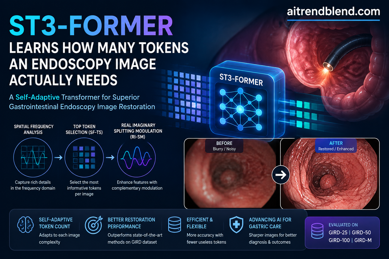
- ST3-Former restores gastrointestinal endoscopy images by letting the network choose its own number of attended tokens per image rather than using a fixed ratio set in advance.
- Two new modules make this possible, Spatial Frequency Token Selection which reads both the spatial and frequency domains to size the token budget, and Real Imaginary Splitting Modulation which treats the real and imaginary parts of the frequency signal separately.
- The authors built and released four Gastrointestinal Image Restoration Datasets covering low resolution images, three levels of synthetic noise, and one set of real world degradations such as motion blur and specular highlights, together totaling 13,378 source images across variants.
- Across ten comparison methods, ST3-Former posted the best PSNR and SSIM scores on every one of the four benchmark datasets, with gains as large as 2.73 decibels in PSNR on the highest noise setting.
- Paired statistical tests on the real world degradation set confirm the improvement is unlikely to be chance, and the model is also faster at inference than its closest rival despite having slightly more parameters.
Why endoscopy images need their own restoration research
Gastric cancer killed 260,372 people in China in a single year according to the 2022 figures the authors cite, trailing only lung and liver cancer as a cause of cancer death in that country. Endoscopy is the frontline tool for catching gastric and intestinal disease early, and a great deal of computer aided diagnosis research assumes the image reaching the algorithm is clean. In practice it rarely is. Motion from the scope, specular highlights off wet mucosal tissue, color distortion from the light source, and compression from the recording pipeline all degrade the image before any diagnostic model ever sees it.
Image restoration as a general field, covering super resolution, denoising and dehazing, is well studied for natural photographs. Endoscopic images are a different animal. They are captured through a narrow lens in an enclosed, wet, oddly lit environment, and the textures a restoration model needs to preserve, small ulcers, faint erythema, the mosaic pattern of bile reflux, are exactly the kind of low contrast detail that aggressive denoising tends to erase along with the noise. The paper’s authors note directly that restoration research specific to gastrointestinal endoscopy has remained limited, which is part of why they built their own benchmark rather than relying on natural image datasets.
The problem with a fixed token budget
The starting point for ST3-Former is a method called TTST, the Top-K Token Selective Transformer, originally built for satellite image super resolution. TTST improves on standard transformer attention by keeping only the top scoring tokens in the attention map and zeroing out the rest, which concentrates the network’s computation on the most informative regions of an image rather than spreading it evenly. The catch is that TTST decides how many tokens to keep using a ratio fixed before training ever starts. Every image, regardless of how much fine detail or how much flat background it contains, gets the same slice of the attention map.
That is a reasonable simplification for a benchmark of similar satellite tiles. It is a poor fit for endoscopy, where one frame might be almost entirely a smooth stomach wall and the next might be packed with polyps, clips, ulcers and visible vessels. A fixed ratio either wastes computation on frames that do not need it or starves detailed frames of the tokens they need to reconstruct fine texture. The authors describe this directly as a limit on generalizability across diverse scenes, and it is the exact problem ST3-Former sets out to fix.
That is the original TTST formulation, where the cutoff ratio \(\alpha_k\) is a constant chosen ahead of time and applied uniformly to the attention map \(\mathcal{M}\). ST3-Former changes exactly one thing in that equation but the change matters a great deal.
Here the cutoff is computed from the attention map itself through the operator \(\alpha_k * \mathcal{M}\), which the authors define as the median of \(\mathcal{M}\) along its spatial dimension, scaled by the factor \(\alpha_k\), then converted into a percentage rank within \(\mathcal{M}\). In plain terms, the network measures how much signal is actually present in this particular image’s attention map and sets its own threshold from that measurement, rather than importing a threshold decided on a different dataset entirely.
Inside ST3-Former, two modules working in tandem
Spatial Frequency Token Selection
The first new module, Spatial Frequency Token Selection, extends the dynamic thresholding idea into the frequency domain as well as the spatial one. The encoder produces feature maps that are converted into query, key and value projections as usual, and an ordinary attention map is computed in the spatial domain. In parallel, that same attention map is passed through a Fourier transform to produce a frequency domain attention map. Both maps go through the same adaptive top token selection process described above, each with its own dynamically computed ratio, and the selected tokens from each domain are summed separately before being carried forward.
The reasoning is that spatial attention and frequency attention notice different things. A blurred edge might still show up clearly as a frequency domain anomaly even when its spatial contrast is too low for ordinary attention to flag it, and the reverse can also be true for texture that is spatially obvious but spectrally unremarkable. Running both selections in parallel and fusing their results lets the network catch degradation patterns that either domain alone would miss.
Real Imaginary Splitting Modulation
The second module addresses something the frequency domain literature does not always take seriously enough. A Fourier transform produces a complex valued signal with a real component and an imaginary component, and most methods that touch the frequency domain treat that complex value as a single unit, often collapsing straight to amplitude and discarding phase information in the process. Real Imaginary Splitting Modulation instead runs the real and imaginary parts through separate convolution and multilayer perceptron branches before recombining them.
The real and imaginary components pass through their own convolution layers, \(f_{c2}\) and \(f_{c3}\), are recombined and inverse transformed back to the spatial domain with \(\Phi^{-1}\), then passed through an amplitude function \(f_{abs}\) before a further convolution and multilayer perceptron refine the result. The ablation study later in the paper is blunt about why this matters, discarding the imaginary component causes a clear, measurable drop in restoration quality, which confirms that phase information the network would otherwise throw away is carrying real signal.
The final fused attention, combining the modulated spatial map, the modulated frequency map, and the original unmodified spatial map as a stabilizing term, is what actually multiplies the value features to produce the output. That third term, the raw \(\mathcal{M}\), is a quiet but important design choice, since it means the modulation modules can only add information on top of the original signal rather than replace it outright.
Where this sits architecturally
ST3-Former does not reinvent the backbone from scratch. It builds on DATNet, a Dual Aggregation Transformer chosen for its computational efficiency, and slots the Spatial Frequency Token Selection and Real Imaginary Splitting Modulation modules into DATNet’s existing spatial and channel self attention blocks. The novelty is concentrated in how tokens are selected and how the frequency signal is processed, not in a wholesale new backbone.
A benchmark built specifically for this problem
Roughly a third of the paper’s contribution is not the model at all, it is the dataset. The authors constructed four Gastrointestinal Image Restoration Datasets, referred to collectively as GIRD, specifically because no existing public benchmark matched the degradation patterns endoscopy actually produces.
GIRD-25, GIRD-50 and GIRD-100 share a common source of 9,922 original images captured at 1024 by 1024 resolution, split into 7,922 training images, 1,000 validation images and 1,000 test images. Each of these three datasets provides a downsampled 256 by 256 low resolution version of every image, with zero mean Gaussian noise added at a standard deviation matching the number in the dataset name, so GIRD-100 is the noisiest of the three. GIRD-M takes a different approach entirely, starting from 5,356 original 320 by 320 images split into 3,658 training, 930 validation and 768 test images, and applying degradations meant to mimic what actually happens during a live procedure, motion blur, light scattering, specular highlights from wet tissue, color distortion and compression artifacts.
The clinical range covered is broad. The source images span patients aged 35 to 72, with findings including post total gastrectomy changes, multiple intestinal polyps, shallow ulcers, resected fundic polyps, duodenal ulcers with a distinctive snowflake pattern, bile reflux, chronic atrophic gastritis, esophageal papilloma and endoscopic submucosal dissection lesions among others. The study received ethical approval from the Institutional Research Ethics Committee of Fuzhou First General Hospital, affiliated with Fujian Medical University, under reference 202209008, dated September 6 2022, and was conducted in compliance with the Declaration of Helsinki with informed consent obtained from participants. The datasets are shared publicly on GitHub, and the authors state the code will be released at a later date.
What the numbers show
ST3-Former was compared against ten established restoration methods, CAMixerSR, TransENet, SwinIR, IMDN, TTST, ESRT, CATANet, DATNet, HiT-SR and SAFMNet, on the combined super resolution and denoising task across GIRD-25, GIRD-50 and GIRD-100.
| Dataset | Metric | Best prior method | ST3-Former |
|---|---|---|---|
| GIRD-25, low noise | PSNR | CAMixerSR, 29.65 dB | 29.99 dB |
| GIRD-25, low noise | SSIM | CAMixerSR, 0.8475 | 0.8945 |
| GIRD-50, moderate noise | PSNR | IMDN, 25.86 dB | 28.59 dB |
| GIRD-100, high noise | PSNR | CAMixerSR, 23.40 dB | 25.37 dB |
| GIRD-100, high noise | SSIM | CAMixerSR, 0.7025 | 0.7789 |
The pattern across increasing noise levels is the most interesting part of this table. Every method’s score falls as noise climbs from GIRD-25 to GIRD-100, which is expected, but the size of the fall varies enormously between methods. TransENet, a comparison method built around a different image restoration approach, collapses from a respectable score on GIRD-25 down to a PSNR of just 13.25 decibels and an SSIM of 0.0583 on GIRD-100, essentially a failure to restore anything usable. ST3-Former’s own decline is far gentler, and the paper frames this specifically as evidence of noise resistance rather than just peak accuracy, which matters more for clinical use than a narrow win on the easiest setting, since a real endoscopy feed will not arrive with a label telling the algorithm how noisy it is.
On GIRD-M, the dataset built from real world degradations rather than synthetic noise, ST3-Former again came out ahead of eight comparison methods including CATANet, HiT-SR, PFT-SR, ESC, AMIR, DASMamba-MedIR, DATNet and FourierSR, scoring 26.67 decibels PSNR and 0.8645 SSIM. The margin here is tighter than on the synthetic noise datasets, and one competitor, ESC, actually posted a marginally higher SSIM of 0.8647 while trailing on PSNR by 0.41 decibels. That kind of near tie on one metric and a clear lead on the other is a more honest picture of real world performance than a clean sweep would be, and it is worth noting plainly rather than glossing over.
ST3-Former demonstrates the slowest rate of decline and the strongest noise resistance. Particularly noteworthy is ST3-Former’s consistent performance preservation across the noise spectrum. Huang, Chen, Lin, Yang, Zheng, Wu and Yang, Knowledge Based Systems, 2026
Confirming the result was not luck
The authors ran three independent training runs on GIRD-100 to check stability, reporting a PSNR of 25.29 plus or minus 0.08 decibels and an SSIM of 0.7834 plus or minus 0.0052 on the test split, with similarly tight spreads on validation. Those are small standard deviations relative to the gap over competing methods, which supports the claim that the improvement is a stable property of the architecture rather than a lucky training run.
More formally, a paired t-test was run comparing ST3-Former against the strongest competing method on GIRD-M. On the test set the t-statistic was 2.8370 with a two sided p value of 0.0047. On the validation set the t-statistic was 3.5953 with a two sided p value of 0.0003. Both results clear the conventional 0.01 and 0.001 significance thresholds respectively, giving the authors grounds to state the improvement is statistically significant rather than within the range of random variation.
What efficiency actually costs, and does not cost
A common assumption is that a more accurate model must be a slower one, and that assumption does not hold up here. Comparing ST3-Former against AMIR, one of its closer performing rivals on GIRD-M, at 320 by 320 input resolution, ST3-Former uses 29.163 million trainable parameters against AMIR’s 23.544 million, a modest increase, and very slightly more floating point operations per image, 198.79 billion against 198.77 billion, essentially a wash. Where the two diverge sharply is inference time. ST3-Former processes a single image in 252.86 milliseconds compared with AMIR’s 545.03 milliseconds, more than twice as fast, while using identical GPU memory of 774 megabytes for both. The dynamic token selection appears to be doing real computational work here, pruning enough of the attention map at inference time to more than offset the extra parameters.
What the ablation study reveals about which piece matters
Removing pieces of ST3-Former one at a time on GIRD-M shows that neither the spatial nor the frequency half of the design is optional.
| Configuration | Validation PSNR | Validation SSIM | Test PSNR | Test SSIM |
|---|---|---|---|---|
| Without spatial domain token selection | 28.33 | 0.8930 | 26.53 | 0.8639 |
| Without frequency domain token selection | 28.23 | 0.8895 | 26.48 | 0.8621 |
| Full ST3-Former | 28.41 | 0.8926 | 26.67 | 0.8645 |
Dropping spatial domain selection hurts test set performance more, which the authors read as evidence that spatial information matters most for generalizing to genuinely unseen data. Dropping frequency domain selection hurts validation performance more, pointing to a role in fine tuning the model during training. Together the two halves of Spatial Frequency Token Selection are doing complementary jobs rather than redundant ones.
A second ablation, isolating pieces of Real Imaginary Splitting Modulation, tells a similarly nuanced story. Removing the stabilizing raw attention term \(\mathcal{M}\) from the final fusion caused only a small validation drop with almost no test set change, suggesting that term contributes but is not load bearing. Discarding the imaginary component of the frequency signal entirely caused a clearer drop on both validation and test sets, confirming the phase information carries real value rather than being an incidental byproduct of the Fourier transform. Replacing the median based threshold statistic with a simple feature mean also underperformed, which the authors attribute to the median having a weaker correlation with the rest of the feature map, making it a cleaner threshold precisely because it is less influenced by outlier values.
A detail worth knowing if you are tuning something similar
The paper’s search over fixed candidate token ratios found that a set of one half, two quarters, three quarters and four fifths outperformed several nearby alternatives on both GIRD-50 and GIRD-M, but the gap between the best and worst tested configuration was under three tenths of a decibel in PSNR. The bigger gain in this paper comes from making the ratio adaptive at all, not from the exact fixed candidates chosen within that adaptive scheme.
The clinical translation gap
It is worth being direct about how far this sits from a deployed clinical tool. The GIRD datasets, however clinically diverse in the pathology they represent, come from a single hospital system in Fujian province, and the low resolution and noisy variants used for three of the four datasets are synthetic degradations applied after the fact rather than genuine sensor limitations captured during live procedures. Only GIRD-M attempts to model real world degradation directly, and it is also the smallest of the four datasets and the one where ST3-Former’s margin over competing methods was narrowest.
Training itself was comparatively brief, twenty epochs on a single NVIDIA Tesla A10 GPU with a batch size of four, which is efficient and reproducible but leaves open how the model would behave on scope models, light sources or patient populations meaningfully different from those represented in the source hospital’s case mix. The authors themselves are the ones who flag the model’s most serious current weakness, and it is worth taking seriously precisely because they did not need to disclose it as clearly as they did.
Honest limitations
The failure cases the authors show are specific and instructive rather than vague. When an endoscopy image suffers from severe blur, particularly when a surgical instrument occupies only a small part of the frame, ST3-Former struggles to recover fine anatomical texture, and the restored instrument itself often comes out geometrically deformed with distorted brightness while small details are effectively lost. The authors attribute this directly to the model having no explicit prior knowledge of what an instrument’s shape and appearance should look like, which makes reconstructing a small, low contrast, heavily blurred object an underconstrained problem for a purely data driven restoration network. Their stated next step is to bring in instrument specific shape priors and dedicated fine detail recovery mechanisms, which is a sensible diagnosis of the actual failure mode rather than a generic promise to keep improving.
A second honest limitation sits in the dataset construction itself. The three noise level datasets rely on synthetic Gaussian noise layered onto otherwise clean high resolution images, which is a standard and defensible benchmarking practice but is not identical to the noise characteristics a real endoscopy sensor produces under variable lighting and motion. The real world degradation set, GIRD-M, is smaller and shows a narrower performance gap, which is itself informative, suggesting the easier synthetic benchmarks may be somewhat flattering relative to genuinely uncontrolled conditions.
Conclusion
The core achievement here is turning a single fixed hyperparameter, the fraction of tokens an attention mechanism keeps, into something the network computes fresh for every image it sees. That sounds like a small technical adjustment, and mechanically it is, but its effect compounds through every layer that uses it, and the ablation results make clear that both the spatial and the frequency version of that adaptive threshold are doing distinct, necessary work rather than duplicating each other.
The conceptual shift worth remembering is that token selection itself became a variable tied to image content rather than a constant tuned once on a validation set and then frozen. That idea does not obviously depend on gastrointestinal endoscopy at all, and the authors’ own baseline comparison, TTST, was originally built for satellite imagery, which suggests the underlying mechanism could transfer to other imaging domains that share the same core problem of highly variable per image detail density, from other endoscopic specialties to dermoscopy to certain classes of remote sensing imagery.
What keeps this grounded rather than overstated is the dataset work sitting alongside the model. Four purpose built benchmarks, released publicly, with a clear split between synthetic and real world degradation, give other researchers a way to check whether ST3-Former’s gains hold up under conditions the original authors did not test, which is exactly the kind of infrastructure a young subfield needs more than another single model claiming a new best score.
The honest remaining limitations, a struggle with small, heavily blurred instruments, a real world degradation set that is smaller and shows a tighter competitive margin than the synthetic ones, and training data drawn from one hospital system, are not minor footnotes. They mark out exactly where the next round of work needs to go, and the authors say so plainly rather than treating the limitations section as a formality.
Read against the wider push toward computer aided gastrointestinal diagnosis, this paper is best understood as groundwork rather than a finished diagnostic tool. A model that cannot see a lesion clearly cannot help characterize it, and by tackling the seeing problem directly, with a released benchmark other teams can build on, ST3-Former earns its place as infrastructure for whatever diagnostic model gets built on top of it next.
A working PyTorch implementation
The block below is a runnable, simplified implementation of the two core modules described in the paper, dynamic top token selection with a median based threshold, Spatial Frequency Token Selection, and Real Imaginary Splitting Modulation, wired into a small transformer block with an L2 training loss, a PSNR and SSIM evaluation function, and a smoke test on random dummy data. It is written to make the mechanics concrete rather than to reproduce the paper’s exact DATNet backbone or its full benchmark numbers, which required the complete GIRD datasets and the paper’s specific training configuration.
# st3former_reference.py
# A compact, runnable reference implementation of the dynamic top token selection,
# Spatial Frequency Token Selection and Real Imaginary Splitting Modulation ideas
# from Huang, Chen, Lin, Yang, Zheng, Wu and Yang, Knowledge Based Systems 2026.
# This is an educational reference, not a reproduction of the paper's exact backbone.

import torch
import torch.nn as nn
import torch.nn.functional as F


def dynamic_top_token_mask(attn, alpha):
    """
    Implements the paper's adaptive threshold, alpha_k * M, using the spatial
    median of the attention map scaled by alpha, converted to a percentage rank
    cutoff. Values below the cutoff are zeroed rather than removed, matching
    the f_top behaviour described around Equation 2 of the paper.
    """
    b, heads, n, m = attn.shape
    flat = attn.reshape(b, heads, -1)
    median = flat.median(dim=-1, keepdim=True).values
    cutoff = alpha * median
    mask = (flat >= cutoff).float()
    masked = flat * mask
    return masked.reshape(b, heads, n, m)


class AdaptiveTopTokenAttention(nn.Module):
    """Standard scaled dot product attention with a self adaptive token cutoff."""

    def __init__(self, dim, heads=4, alpha=0.5):
        super().__init__()
        self.heads = heads
        self.head_dim = dim // heads
        self.scale = self.head_dim ** -0.5
        self.alpha = alpha

        self.to_q = nn.Linear(dim, dim)
        self.to_k = nn.Linear(dim, dim)
        self.to_v = nn.Linear(dim, dim)
        self.out_proj = nn.Linear(dim, dim)

    def forward(self, x):
        b, n, c = x.shape
        q = self.to_q(x).view(b, n, self.heads, self.head_dim).transpose(1, 2)
        k = self.to_k(x).view(b, n, self.heads, self.head_dim).transpose(1, 2)
        v = self.to_v(x).view(b, n, self.heads, self.head_dim).transpose(1, 2)

        attn = torch.matmul(q, k.transpose(-2, -1)) * self.scale
        attn = dynamic_top_token_mask(attn, self.alpha)
        attn = F.softmax(attn, dim=-1)

        out = torch.matmul(attn, v)
        out = out.transpose(1, 2).reshape(b, n, c)
        return self.out_proj(out)


class RealImaginarySplittingModulation(nn.Module):
    """
    Splits a frequency domain attention map into real and imaginary parts,
    modulates each with its own convolution branch, then recombines them
    following the structure of Equation 6 in the paper.
    """

    def __init__(self, dim):
        super().__init__()
        self.conv_real = nn.Conv2d(dim, dim, kernel_size=3, padding=1)
        self.conv_imag = nn.Conv2d(dim, dim, kernel_size=3, padding=1)
        self.conv_out = nn.Conv2d(dim, dim, kernel_size=3, padding=1)
        self.mlp_out = nn.Sequential(
            nn.Linear(dim, dim * 2),
            nn.GELU(),
            nn.Linear(dim * 2, dim),
        )

    def forward(self, feature_map):
        # feature_map: b, c, h, w in the spatial domain
        freq = torch.fft.fft2(feature_map, norm="ortho")
        real_part = self.conv_real(freq.real)
        imag_part = self.conv_imag(freq.imag)

        recombined = torch.complex(real_part, imag_part)
        spatial_back = torch.fft.ifft2(recombined, norm="ortho")
        amplitude = torch.abs(spatial_back)

        refined = self.conv_out(amplitude)
        b, c, h, w = refined.shape
        tokens = refined.flatten(2).transpose(1, 2)
        tokens = self.mlp_out(tokens)
        return tokens.transpose(1, 2).reshape(b, c, h, w)


class SpatialFrequencyTokenSelection(nn.Module):
    """
    Runs adaptive top token attention in parallel on the spatial feature map
    and on its frequency domain magnitude, then fuses both selections with
    Real Imaginary Splitting Modulation.
    """

    def __init__(self, dim, heads=4, alpha=0.5):
        super().__init__()
        self.spatial_attn = AdaptiveTopTokenAttention(dim, heads, alpha)
        self.freq_attn = AdaptiveTopTokenAttention(dim, heads, alpha)
        self.ri_sm = RealImaginarySplittingModulation(dim)
        self.proj = nn.Linear(dim, dim)

    def forward(self, feature_map):
        b, c, h, w = feature_map.shape
        tokens = feature_map.flatten(2).transpose(1, 2)

        spatial_out = self.spatial_attn(tokens)

        freq_map = torch.fft.fft2(feature_map, norm="ortho")
        freq_amplitude = torch.abs(freq_map)
        freq_tokens = freq_amplitude.flatten(2).transpose(1, 2)
        freq_out = self.freq_attn(freq_tokens)

        modulated = self.ri_sm(feature_map)
        modulated_tokens = modulated.flatten(2).transpose(1, 2)

        fused = spatial_out + freq_out + modulated_tokens
        fused = self.proj(fused)
        return fused.transpose(1, 2).reshape(b, c, h, w)


class ST3FormerBlockLite(nn.Module):
    """A single transformer block combining SF-TS with a lightweight feed forward path."""

    def __init__(self, dim, heads=4, alpha=0.5):
        super().__init__()
        self.norm1 = nn.GroupNorm(1, dim)
        self.sf_ts = SpatialFrequencyTokenSelection(dim, heads, alpha)
        self.norm2 = nn.GroupNorm(1, dim)
        self.ffn = nn.Sequential(
            nn.Conv2d(dim, dim * 2, kernel_size=1),
            nn.GELU(),
            nn.Conv2d(dim * 2, dim, kernel_size=1),
        )

    def forward(self, x):
        x = x + self.sf_ts(self.norm1(x))
        x = x + self.ffn(self.norm2(x))
        return x


class ST3FormerLite(nn.Module):
    """A small end to end restoration network built from ST3FormerBlockLite blocks."""

    def __init__(self, in_channels=3, dim=32, depth=3, heads=4, alpha=0.5):
        super().__init__()
        self.stem = nn.Conv2d(in_channels, dim, kernel_size=3, padding=1)
        self.blocks = nn.ModuleList(
            [ST3FormerBlockLite(dim, heads, alpha) for _ in range(depth)]
        )
        self.head = nn.Conv2d(dim, in_channels, kernel_size=3, padding=1)

    def forward(self, degraded_image):
        feat = self.stem(degraded_image)
        for block in self.blocks:
            feat = block(feat)
        residual = self.head(feat)
        return degraded_image + residual


def restoration_loss(pred, target):
    # Matches the L2 norm loss used to train ST3-Former, Equation 9 of the paper.
    return F.mse_loss(pred, target, reduction="sum") / pred.shape[0]


def compute_psnr(pred, target, max_value=1.0):
    mse = F.mse_loss(pred, target)
    if mse.item() == 0:
        return float("inf")
    return (10 * torch.log10((max_value ** 2) / mse)).item()


def compute_ssim(pred, target, c1=(0.01 * 1.0) ** 2, c2=(0.03 * 1.0) ** 2):
    """A simplified single scale SSIM over the whole image, for smoke testing only."""
    mu_pred = pred.mean(dim=(2, 3), keepdim=True)
    mu_target = target.mean(dim=(2, 3), keepdim=True)

    var_pred = pred.var(dim=(2, 3), keepdim=True, unbiased=False)
    var_target = target.var(dim=(2, 3), keepdim=True, unbiased=False)
    covar = ((pred - mu_pred) * (target - mu_target)).mean(dim=(2, 3), keepdim=True)

    numerator = (2 * mu_pred * mu_target + c1) * (2 * covar + c2)
    denominator = (mu_pred ** 2 + mu_target ** 2 + c1) * (var_pred + var_target + c2)
    ssim_map = numerator / denominator
    return ssim_map.mean().item()


def train_one_step(model, optimizer, degraded, clean):
    model.train()
    optimizer.zero_grad()
    restored = model(degraded)
    loss = restoration_loss(restored, clean)
    loss.backward()
    optimizer.step()
    return loss.item()


@torch.no_grad()
def evaluate(model, degraded, clean):
    model.eval()
    restored = model(degraded).clamp(0, 1)
    psnr = compute_psnr(restored, clean)
    ssim = compute_ssim(restored, clean)
    return psnr, ssim


def smoke_test():
    """Runs one training step and one evaluation step on random dummy data."""
    device = torch.device("cuda" if torch.cuda.is_available() else "cpu")
    torch.manual_seed(0)

    batch_size, channels, height, width = 2, 3, 64, 64
    clean = torch.rand(batch_size, channels, height, width, device=device)
    noise = torch.randn_like(clean) * 0.05
    degraded = (clean + noise).clamp(0, 1)

    model = ST3FormerLite(in_channels=channels, dim=32, depth=2, heads=4, alpha=0.5).to(device)
    optimizer = torch.optim.Adam(model.parameters(), lr=1e-4)

    loss_value = train_one_step(model, optimizer, degraded, clean)
    psnr, ssim = evaluate(model, degraded, clean)

    print(f"Smoke test training loss {loss_value:.4f}")
    print(f"Smoke test PSNR {psnr:.4f} dB")
    print(f"Smoke test SSIM {ssim:.4f}")
    assert torch.isfinite(torch.tensor(loss_value))
    print("Smoke test passed")


if __name__ == "__main__":
    smoke_test()
Frequently asked questions
What does ST3-Former stand for and what task does it perform
ST3-Former stands for Self adaptive Top Token Transformer. It restores gastrointestinal endoscopy images, handling super resolution and denoising together on the GIRD-25, GIRD-50 and GIRD-100 datasets and general real world restoration on GIRD-M.
Is ST3-Former a diagnostic tool
No. It restores image quality, it does not diagnose disease. Nothing in the paper claims diagnostic authority, and any clinical use would need separate validation, regulatory clearance and oversight by qualified professionals.
How is this different from the earlier TTST method it builds on
TTST selects a fixed, pre chosen fraction of attention tokens for every image. ST3-Former computes that fraction fresh for each image from the attention map’s own median value, which the ablation study shows improves generalization to varied image content.
What are the four GIRD datasets
GIRD-25, GIRD-50 and GIRD-100 share the same 9,922 source images with low resolution versions and Gaussian noise at three severity levels. GIRD-M contains 5,356 separate images degraded with motion blur, light scattering, specular highlights, color distortion and compression artifacts to approximate real world conditions.
Is the improvement over prior methods statistically meaningful
The authors ran paired t-tests on the GIRD-M dataset. The test set comparison produced a two sided p value of 0.0047 and the validation set comparison produced a two sided p value of 0.0003, both below conventional significance thresholds.
Where does the model still struggle
The authors report that severely blurred images, especially ones where a surgical instrument occupies a small part of the frame, are reconstructed poorly, with visible geometric deformation and brightness distortion in the instrument itself.
Read the full paper for the complete equations, all ten comparison methods and the released dataset.
Read the paper on Knowledge Based Systems GIRD datasets on GitHubRelated reading
Academic citation. Huang, Y., Chen, Y., Lin, H., Yang, M., Zheng, X., Wu, Y. and Yang, K. A self adaptive top token transformer for gastrointestinal endoscopy image restoration. Knowledge Based Systems, 349, 116445, 2026. https://doi.org/10.1016/j.knosys.2026.116445
This analysis is based on the published paper and an independent evaluation of its claims.