Sheffer Sequences With Zeros on a Line — A Hidden Bridge to the Riemann Zeta Function | AI Trend Blend

Pure Mathematics · Journal of Mathematical Analysis and Applications 563 (2026) · Sungkyunkwan University & California State University, Fresno · 14 min read

Zeros in Perfect Formation — How a Family of Polynomials Lines Up on a Single Vertical Line, and What That Has to Do With the Riemann Zeta Function

A three-author research team spanning South Korea and California has proved that a sweeping family of Sheffer polynomial sequences has virtually all of its zeros pinned to one vertical line in the complex plane — and along the way discovered a quiet, beautiful link to the Riemann zeta function that no one had seen before.

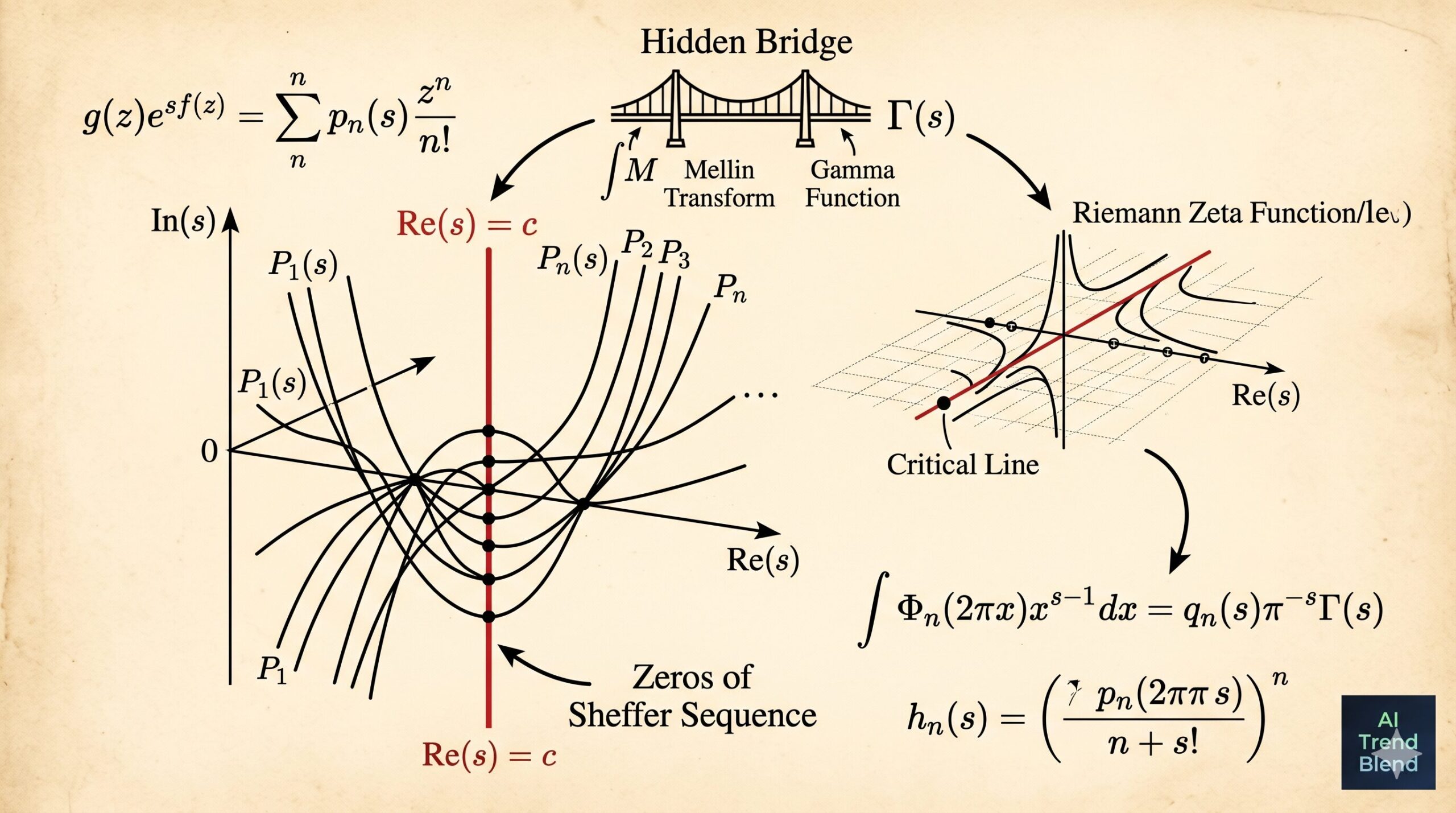
Sheffer Sequences Zeros on a Line Riemann Zeta Function Mellin Transform Laguerre Polynomials Meixner Polynomials Riordan Matrices Saddle Point Method

Imagine plotting the roots of a degree-ten polynomial in the complex plane and watching them all snap into a single perfectly straight vertical column. Now imagine proving that this happens not just for one polynomial, but for every polynomial in an infinite sequence — and not just for one sequence, but for an enormous family of them generated by a flexible two-parameter formula. That, in essence, is what this paper accomplishes. And tucked inside the proof is an unexpected identity that connects these polynomials directly to the Riemann zeta function.

What Is a Sheffer Sequence, and Why Should You Care About Its Zeros?

Before diving into the mathematics, it helps to understand what we mean by a Sheffer sequence. In combinatorics and analysis, a Sheffer sequence is a family of polynomials $\{p_n(s)\}_{n \geq 0}$ — one polynomial of degree $n$ for each non-negative integer $n$ — whose generating function can be written in the compact exponential form

Sheffer Generating Function $$g(z)\,e^{s f(z)} = \sum_{n=0}^{\infty} p_n(s)\,\frac{z^n}{n!}$$

for two power-series functions $g(z)$ and $f(z)$. This is an incredibly rich class of objects: the Hermite polynomials, the Laguerre polynomials, the Bernoulli polynomials, and many other classical families all belong to it. Sheffer sequences appear in combinatorics (counting problems), probability (moment generating functions), numerical analysis (interpolation), and mathematical physics (quantum mechanics). Understanding their structure — including where their zeros live in the complex plane — has real consequences across all of these fields.

The specific question this paper attacks is: when can you guarantee that the zeros of every polynomial in the sequence lie on a single vertical line $\mathrm{Re}(s) = c$ in the complex plane? This is a strong, elegant property. It means that however large the degree grows, the roots never scatter across the plane — they stay disciplined, organized along a fixed axis. Proving it requires both algebraic structure (the right generating function form) and hard asymptotic analysis (controlling the behavior of complex integrals as degree $n \to \infty$).

The Central Question in Plain Language

You have an infinite list of polynomials — one of degree 1, one of degree 2, one of degree 3, and so on — all generated by the same formula. The question is: can you prove that the roots of every one of these polynomials lie on the same vertical line in the complex plane? This paper says yes — for a huge family of such generating formulas — and tells you exactly which vertical line they land on.

The Starting Point — What Bump et al. Proved, and What This Paper Extends

The story begins with a 2000 result by Bump, Choi, Kurlberg, and Vaaler, who studied the Mellin transforms of the so-called Laguerre functions. The Laguerre functions are defined by

Laguerre Functions $$\mathfrak{L}_n^{(\alpha)}(x) = x^{\alpha/2} e^{-x/2} L_n^{(\alpha)}(x), \quad \alpha > -1,$$

where $L_n^{(\alpha)}(x)$ are the classical generalized Laguerre polynomials. When you take the Mellin transform of $\mathfrak{L}_n^{(\alpha)}$, you get an expression of the form $2^{s+\alpha/2}\Gamma(s+\alpha/2)P_n^{(\alpha)}(s)$, where the polynomials $P_n^{(\alpha)}(s)$ are generated by the two-factor product

Bump Generating Function $$\sum_{n=0}^{\infty} P_n^{(\alpha)}(s)\,z^n = (1-z)^{s-1-\alpha/2}(1+z)^{-s-\alpha/2}.$$

Bump et al. proved that the zeros of every polynomial $P_n^{(\alpha)}(s)$ lie on the critical line $\mathrm{Re}(s) = \tfrac{1}{2}$. This is not a coincidence — there is a deep structural reason for it rooted in a symmetry of the generating function. And it hinted at a possible connection to the Riemann hypothesis, since the critical line $\mathrm{Re}(s) = \tfrac{1}{2}$ is precisely the line where the Riemann zeta function is conjectured to have all of its non-trivial zeros.

The main theorem of the present paper generalizes Bump’s result from one specific generating function to a whole parametric family. Instead of the two-factor product above, Cheon, Forgács, and Tran consider generating functions of the form

Generalized Generating Function (Theorem 1) $$\sum_{n=0}^{\infty} h_n(s)\,\frac{z^n}{n!} = (1-\alpha_0 z)^{p+s}(1+\alpha_0 z)^{p^*-s} \prod_{i=1}^{N}(1-\alpha_i^2 z^2)^{p_i},$$

where $\alpha_0, \alpha_1, \ldots, \alpha_N$, $p$, $p^*$, and $p_1, \ldots, p_N$ are real parameters, and the $\alpha_i$ are distinct in absolute value. Bump’s specific result is recovered as the very special case $N = 0$, $\alpha_0 = 1$, $p = -1 – \alpha/2$, $p^* = -\alpha/2$.

Theorem 1 — Main Zero-Line Result

Let $\{h_n(s)\}$ be defined by the generating function above. If $p^* + p \leq 0$, then for every $n$, all zeros of $h_n(s)$ lie on the vertical line $\mathrm{Re}(s) = (p^*-p)/2$.

If $p^* + p > 0$, the same conclusion holds except for at most $2\lceil c + p \rceil$ zeros, where $c = (p^*-p)/2$.

The condition $p^* + p \leq 0$ is natural: it ensures a precise symmetry of the generating function under a specific functional equation, which is what forces the zeros onto the line. When $p^* + p > 0$, a finite number of zeros are allowed to stray, but the rest — infinitely many, growing without bound — remain perfectly aligned.

The Intermediate Polynomials — A Sequence With Its Own Life

One of the most elegant ideas in the paper is the introduction of an intermediate polynomial sequence $\{q_n(s)\}$, generated by simply zeroing out the product term in the generating function:

Intermediate Sequence $$\sum_{n=0}^{\infty} q_n(s)\,\frac{z^n}{n!} = (1 – z)^{p+s}(1+z)^{p^*-s}.$$

These $q_n$ polynomials are the direct generalization of Bump’s $P_n^{(\alpha)}$ — they are the “core” of the family, without the extra product factors. The authors show that the full polynomials $h_n(s)$ can be expressed explicitly as weighted sums of the $q_k(s)$:

$h_n(s) = \sum_{k=0}^n \frac{n!}{k!}\, b_{n-k}\, q_k(s),$

where the $b_k$ are the Taylor coefficients of the product $\prod_{i=1}^N (1-\alpha_i^2 z^2)^{p_i}$. This decomposition, derived using the algebraic framework of Riordan matrices, reduces the problem of understanding $h_n$ to understanding $q_n$ — and the $q_n$ have much cleaner properties.

Among those clean properties: the $q_n$ satisfy a functional equation $q_n(s) = (-1)^n q_n(p^* – p – s)$, which mirrors the classical functional equation of the Riemann zeta function. When $p^* – p = 1$, this becomes $q_n(s) = (-1)^n q_n(1-s)$ — exactly the symmetry the zeta function has about the critical line $\mathrm{Re}(s) = \tfrac{1}{2}$.

“The polynomials $q_n(s)$ satisfy the functional equation $q_n(s) = (-1)^n q_n(p^* – p – s)$, which is a standard result in the theory of the zeta function. In particular, if $p^* – p = 1$, then $q_n(s) = (-1)^n q_n(1-s)$.” — Cheon, Forgács, Tran · J. Math. Anal. Appl. 563 (2026)

The $q_n$ also satisfy two distinct recurrence relations, both derived in the paper. A four-term recurrence links $q_{n+1}(s)$ to $q_n(s)$, $q_n(s+1)$, and $q_n(s-1)$. A cleaner three-term recurrence — analogous to the classical recurrences satisfied by orthogonal polynomials — links $q_{n+1}(s)$ directly to $q_n(s)$ and $q_{n-1}(s)$:

Three-Term Recurrence $$q_{n+1}(s) = (p^* – p – 2s)\,q_n(s) + n(n – p^* – p – 1)\,q_{n-1}(s).$$

This three-term recurrence is what drives the interlacing result for the zeros of the $q_n$ sequence — a beautiful structural property saying that the zeros of consecutive polynomials alternate on the vertical line, each polynomial’s zeros separating those of the previous one.

Zeros That Interlace — Structure on the Vertical Line

The zero-on-a-line result is striking enough on its own. But the paper goes further by showing that the zeros do not just sit on the line — they interlace. The zeros of $q_n(s)$ and $q_{n+1}(s)$ alternate along the line, each separating consecutive zeros of the other, in a pattern exactly analogous to what happens with zeros of orthogonal polynomials on the real line.

The proof of interlacing uses the three-term recurrence and a general algebraic lemma about polynomials: if two polynomials of consecutive degree interlace, and a third is formed from them by a recurrence with the right sign condition, then the third interlaces with the second. The condition $p^* + p \leq 0$ — which appeared earlier as the condition for all zeros to lie on the line — also turns out to be exactly the condition needed for the coefficient in the recurrence to have the right sign. The two conditions are not independent: they come from the same structural property of the generating function.

What Interlacing Means

Think of the zeros of $q_n(s)$ as n points on a vertical line, listed from top to bottom. The interlacing property says that the zeros of $q_{n+1}(s)$ — one more in total — slip in between those of $q_n(s)$, with one at each end. It is a kind of perfect democratic spacing that grows more refined with every new polynomial in the sequence.

The Zeta Connection — A Scaled Mellin Transform Identity

The most surprising result in the paper is a direct connection between the polynomial sequence $\{q_n(s)\}$ and the Riemann zeta function $\zeta(s)$. The connection runs through Mellin transforms.

The authors define a family of functions $\Phi_n(s)$ by performing an umbral composition of an Appell sequence with the Laguerre polynomials, and multiplying by $e^{-s/2}$. The resulting functions are combinations of products of Laguerre polynomials with exponential weights. They then prove the following integral identity:

Theorem 9 — Mellin Transform Identity

For every $n \geq 0$,

$$\int_0^\infty \Phi_n(2\pi x)\,x^{s-1}\,dx = q_n(s)\,\pi^{-s}\,\Gamma(s).$$

The Mellin transform of $\Phi_n(2\pi\,\cdot\,)$ factors as the polynomial $q_n(s)$ times the standard Gamma function factor $\pi^{-s}\Gamma(s)$.

In other words, the scaled Mellin transform of these Laguerre-based functions is essentially the polynomial $q_n(s)$, with no extra complications. This is a strikingly clean factorization — and it becomes even more powerful when combined with the definition of the zeta function.

The authors go one step further. They define a function $\psi_j^*(x) = \sum_{n=1}^\infty \Phi_j^*(n\sqrt{x})$, where $\Phi_j^*$ is a re-scaled version of $\Phi_j$, and prove:

Theorem 11 — The Zeta Connection

For every $j \geq 0$,

$$\int_0^\infty \psi_j^*(x)\,x^{s/2-1}\,dx = q_j(s/2)\,\pi^{-s/2}\,\Gamma(s/2)\,\zeta(s).$$

The Mellin transform of $\psi_j^*$ is the product of the polynomial $q_j(s/2)$, the Gamma factor $\pi^{-s/2}\Gamma(s/2)$, and the Riemann zeta function $\zeta(s)$.

This identity is not just a curiosity. It means that understanding the zeros of the scaled Mellin transform on the left-hand side is equivalent to understanding the zeros of the product $q_j(s/2)\cdot\zeta(s)$ on the right. The zeros of $q_j(s/2)$ are precisely the points $s = 2(c + ir)$ where $r$ is a zero of $q_j$ on its vertical line — and by Theorem 1, all of those zeros are controlled. The zeros of $\zeta(s)$ are, of course, exactly the zeros of the Riemann zeta function. So this identity entangles the two, suggesting that studying these polynomial Mellin transforms might one day offer a new approach to zeta-function questions.

The Proof Engine — Saddle Point Asymptotics on a Contour

The proof of Theorem 1 is where the real technical heaviness lives. The strategy is classical but demanding: represent the polynomials via a contour integral using Cauchy’s differentiation formula, deform the contour to pass through a saddle point, develop uniform asymptotic approximations of the integral on two overlapping ranges of the parameter $t$, and then count zeros using the argument principle.

More concretely, the polynomial $h_n(c – int)$ — where $t$ is a real variable and $c = (p^*-p)/2$ — is expressed as a contour integral, which is then rewritten as an integral $p_n(t)$ over a Hankel contour looping around the cut $[1, \infty)$. The saddle point $\zeta(t) = -it + \sqrt{1-t^2}$ lies on the unit circle in the fourth quadrant for $t \in (0,1)$.

Regime 1: Small t (near zero)

When $t = \mathcal{O}(\log^4 n / n)$, the integral is approximated by a Hankel contour asymptotics involving the Gamma function: $p_n(t) \sim i\sin\pi(c+p+1-int)\,\Gamma(c+p+1-int)\cdot(\text{explicit factor})$. This range covers the part of the zero distribution close to the real axis.

Regime 2: t bounded away from 0

When $\log^4 n / n \ll t < 1$, the saddle point method gives $p_n(t) \sim \psi(\zeta)\,e^{n\phi(\zeta,t)}\int_{-\epsilon}^{\epsilon} e^{-ny^2}z'(y)\,dy$, where $z(y)$ is a carefully constructed analytic curve through the saddle. The argument principle on this expression counts the zeros in each strip.

One of the most technically involved parts of the proof is showing that the contour deformation is valid — that the curve $z(y)$ through the saddle point exists, is analytic on a neighborhood of $(-\infty, L)$ for some $L \in (0,1)$, and lies entirely in the fourth quadrant away from the cut. This requires the authors to rule out, one by one, all possible obstructions: the curve cannot hit the negative imaginary axis, cannot return to the unit circle at a second point, and must exit through the real segment $(0,1)$. The proof runs through a careful application of the Mean Value Theorem, a Lagrange multiplier calculation, and a computer-algebra-aided verification of a polynomial inequality.

The limiting zero distribution density is also computed explicitly. As $n \to \infty$, the zeros of $h_n(c – int)$ become dense on the vertical line $\mathrm{Re}(s) = c$, with a density function given by

Limiting Density Function $$D(x) = \frac{1}{2\pi}\ln\frac{1 + \sqrt{1 – x^2}}{1 – \sqrt{1 – x^2}}, \quad x \in (0, 1).$$

This is an arcsine-like distribution that is symmetric about $x = 0$, with density concentrating near $x = 0$ (i.e., near the real axis) and thinning as $x \to \pm 1$. It is a universal feature of the entire family, independent of the specific parameters $p$, $p^*$, and the $\alpha_i$.

The Algebraic Backbone — Riordan Matrices and Umbral Composition

Before the saddle-point analysis can be set up, the algebraic framework needs to be established. This is where the paper deploys the theory of Riordan matrices — a powerful bookkeeping device for sequences and generating functions in combinatorics.

A key insight is that the generating function of $\{h_n(s)\}$ factors, via the Riordan product, as the composition of the “core” generating function for $\{q_n(s)\}$ with the exponential Riordan matrix corresponding to the product factors $\prod (1 – \alpha_i^2 z^2)^{p_i}$. This factorization is what gives the explicit formula expressing $h_n$ as a weighted sum of the $q_k$, and it is what allows all the hard analytic work to be concentrated on $q_n$ alone.

The Meixner polynomials also make a surprise appearance. Using the umbral calculus, the authors express the $q_n$ in terms of Meixner polynomials $\mathfrak{M}_k(-s; -p, -1)$. This representation, combined with a known Mellin transform identity for Laguerre functions, is exactly what makes the proof of Theorem 9 work: the Mellin transform of $\Phi_n(2\pi x)$ can be evaluated term by term using the Meixner representation, and the result collapses to $q_n(s)\,\pi^{-s}\,\Gamma(s)$.

Why the Algebra Matters

The proof is not purely analytic — it rests on a careful algebraic decomposition of the generating function using Riordan matrices, which converts a hard problem about a complicated family into a clean problem about a simpler “core” family. The saddle-point analysis then closes the argument by controlling the asymptotics of that simpler family. Neither half of the proof would work without the other.

Connections, Context, and What Comes Next

This paper sits at the intersection of several mathematical traditions. The zero-on-a-line question connects directly to the Pólya-Schur theory and the Laguerre-Pólya class of entire functions — a deep body of work characterizing functions that are limits of polynomials with only real zeros. The functional equation satisfied by $q_n$ echoes the functional equation of the Riemann zeta function. And the Mellin transform identity in Theorem 11 provides a concrete integral representation that intertwines polynomial zeros and zeta zeros in a single equation.

The authors note that similar techniques could be applied to other generalized Sheffer-type polynomial families — including the Sheffer-Bernoulli, Sheffer-Euler, Laguerre-Appell, and Legendre-Sheffer families that have been studied by other researchers. The key requirement is that the generating function has the right symmetry under the substitution $s \mapsto p^* – p – s$. When that symmetry is present, the zeros are forced onto the vertical line $\mathrm{Re}(s) = (p^*-p)/2$; when it is slightly violated (as in the $p^* + p > 0$ case), only a controlled finite number of zeros can escape.

From a broader perspective, results like this contribute to a growing body of evidence that the structure of polynomial zeros is not random — that generating functions with special symmetries produce zero distributions with special geometric properties. The hope, voiced cautiously in this literature, is that a better understanding of these polynomial analogs might eventually shed light on the Riemann hypothesis itself. The identity in Theorem 11 does not resolve the hypothesis, but it does establish a precise algebraic relationship between a family of polynomials whose zeros are fully understood and the zeta function whose zeros remain the deepest open problem in mathematics.

Read the Full Paper

Published in the Journal of Mathematical Analysis and Applications, Volume 563 (2026). The complete proofs, asymptotic calculations, and Appendix are available via the journal’s website.

📄 Read the Paper (DOI) 🔗 JMAA Journal Page

Academic Citation:
G.-S. Cheon, T. Forgács, K. Tran. Sheffer sequences with zeros on a line. Journal of Mathematical Analysis and Applications, 563 (2026) 130783. https://doi.org/10.1016/j.jmaa.2026.130783

This article is an independent editorial analysis of a peer-reviewed open-access paper published under the CC BY-NC-ND 4.0 license. Mathematical statements paraphrase the original results; for complete proofs and precise formulations, consult the published paper. The paper was received August 7, 2025, and made available online May 7, 2026.

References

[1] G.E. Andrews, R. Askey, R. Roy. Special Functions. Cambridge University Press, 1999.
[2] M.K. Atakishiyeva, N.M. Atakishiyev. On the Mellin transform of hypergeometric polynomials. J. Phys. A, Math. Gen. 32 (1999) L33–L41.
[3] D. Bump, E.K.-S. Ng. On Riemann’s zeta function. Math. Z. 192 (1986) 195–204.
[4] D. Bump, K.-K. Choi, P. Kurlberg, J. Vaaler. A local Riemann hypothesis, I. Math. Z. 233 (2000) 1–19.
[5] G.-S. Cheon, T. Forgács, K. Tran. On the zeros of certain Sheffer sequences and their cognate sequences. Forthcoming in Rocky Mountain J. Math.
[6] G.-S. Cheon, T. Forgács, A. Mwfase, K. Tran. On combinatorial properties and the zero distribution of certain exponential Sheffer sequences. J. Math. Anal. Appl. (2024) 128513.
[7] G.-S. Cheon, T. Forgács, H. Kim, K. Tran. On combinatorial properties and the zero distribution of certain Sheffer sequences. J. Math. Anal. Appl. 514(1) (2022).
[8] S. Khan, N. Raza. Families of Legendre-Sheffer polynomials. Math. Comput. Model. 55 (2012) 969–982.
[9] S. Khan, M. Riyasat. A determinantal approach to Sheffer-Appell polynomials via monomiality principle. J. Math. Anal. Appl. 421(1) (2015) 806–829.
[10] L.L. Liu, Y. Wang. A Unified Approach to Polynomial Sequences with Only Real Zeros. Adv. in Appl. Math. 38 (2007) 542–560.
[11] R.B. Paris. The asymptotics of the Mittag-Leffler polynomials. J. Class. Anal. 1(1) (2012) 1–16.
[12] A.D. Polyanin, A.V. Manzhirov. Handbook of Mathematics for Engineers and Scientists. Chapman & Hall/CRC, 2007.
[13] S. Roman. The theory of the Umbral Calculus I. J. Math. Anal. Appl. 87(1) (1982).
[14] L. Shapiro, R. Sprugnoli, P. Barry, G.-S. Cheon, T.-X. He, D. Merlini, W. Wang. The Riordan Group and Applications. Springer Monographs in Mathematics, 2022.