
Key points
- DeepCut++ extends a prior graph neural network method called DeepCut by adding a Personalized PageRank diffusion module and a multi scale feature fusion step, both aimed at fixing DeepCut’s inability to connect distant, similar regions of an image.
- Across five benchmark datasets covering object localization, single object segmentation, and semantic part segmentation, DeepCut++ posts the best published score against twenty four prior methods.
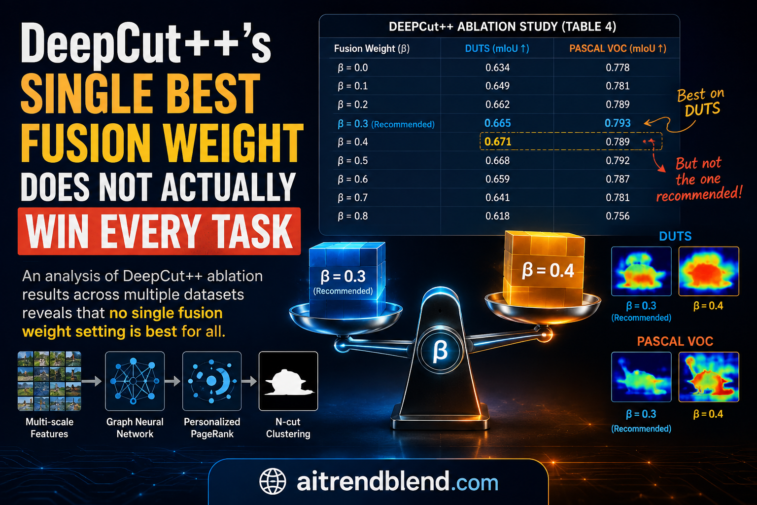
- The paper’s own ablation study on the feature fusion weight, tested across five settings, shows the recommended configuration losing to a different setting on the DUTS dataset specifically.
- All evaluation is done with no training split at all, each image is processed independently at test time, which changes what these numbers can and cannot tell you about generalization.
- The fusion weights themselves are fixed by hand rather than learned, a limitation the authors name directly in their own conclusion.
What problem this is actually solving
Unsupervised image segmentation asks a model to draw meaningful boundaries around objects in a photo without ever being told what those objects are. No labeled training data, no annotated masks, just pixels in and a partition of the image out. It sounds almost impossible, and for a long time it mostly was, with early approaches falling back on thresholding by color intensity or growing regions outward from seed pixels, both of which fall apart the moment an image has a busy background, uneven lighting, or an object that blends into its surroundings.
Graph based methods took a different route. Instead of reasoning pixel by pixel, they represent the image as a graph, where each node is a small patch of the image and each edge carries a weight describing how similar two patches are. Segmentation then becomes a graph partitioning problem, splitting the graph into groups of nodes that are internally similar and mutually dissimilar across groups. This framing has real advantages. It naturally handles irregular object shapes, and it lets a global cost function balance local detail against the overall structure of the image rather than making greedy local decisions the way region growing does.
The specific predecessor this paper builds on, called DeepCut, combined a pretrained vision transformer with a lightweight graph neural network trained using classical clustering objectives. It worked well enough to beat a long list of earlier unsupervised methods. But it had a structural weakness that the DeepCut++ authors focus their entire contribution on fixing. DeepCut’s graph neural network only passes information between directly connected nodes. Two patches that belong to the same object but sit far apart in the image, say the head and the tail of a bird separated by open background, never directly influence each other. The result is that large or oddly shaped objects can end up segmented into disconnected pieces, and any local noise in the pixel features has nowhere to be smoothed away.
The two fixes DeepCut++ adds
A diffusion process borrowed from web search ranking
The centerpiece of DeepCut++ is Personalized PageRank, a technique with an unlikely origin story. It descends from the algorithm Google originally used to rank web pages, adapted here to rank and smooth relationships between graph nodes instead of web pages. The idea the authors lean on is that PPR functions as a low pass filter for node features. High frequency variation, the kind that shows up as noisy or spurious differences between neighboring patches, gets suppressed, while the low frequency structure that actually defines a coherent region gets preserved and even amplified.
The mechanism that makes this work is a teleportation term. At each step of the diffusion process, a node’s updated feature is a weighted mix of information gathered from its graph neighbors and a small amount of its own original feature, controlled by a parameter alpha between zero and one.
That teleportation term is what gives the method its long range reach. Because every node retains a path back to itself, information can effectively hop across the graph over multiple diffusion steps rather than being limited to whatever a node’s immediate neighbors happen to be. The authors argue this is exactly what DeepCut was missing, a way for a bird’s head and tail, connected only through a chain of intermediate patches, to eventually influence each other’s feature representation even though they are never directly linked in the graph.
After computing this PPR matrix, the authors combine it with the original affinity matrix through element wise multiplication rather than replacing it outright.
This keeps the diffusion process anchored to the actual similarity structure of the image. A pair of nodes only gets a strong combined weight if they are both well connected through the diffusion process and genuinely similar according to the original affinity matrix. Weak or noisy connections get attenuated from both directions at once.
Combining two layers of a vision transformer instead of one
The second contribution is more straightforward. Rather than using features from only the final layer of the pretrained DINO vision transformer, as DeepCut does, DeepCut++ pulls features from an intermediate layer, the sixth of eleven, and combines them with the final layer’s output.
The reasoning is that different depths of a vision transformer encode different kinds of information. Middle layers tend to carry richer mid level detail, edges, textures, and local structure, while the final layer has been compressed toward high level, object centric semantics through the additional transformer blocks it passed through. Fusing the two is meant to give the graph nodes access to both fine spatial detail and broad semantic identity at once, which should help the model draw boundaries that are both semantically correct and spatially precise.
How the whole pipeline fits together
Putting the pieces in order, DeepCut++ runs in four stages. First, the frozen DINO backbone extracts patch level features from both the sixth and eleventh transformer blocks. Second, the feature fusion module blends those two feature sets into a single representation per patch using the weighted average from equation 7. Third, a graph is constructed where each patch is a node and edge weights come from the cosine similarity between fused feature vectors, formalized as the affinity matrix W equal to F times F transpose, with negative similarities clipped to zero since the clustering objective used downstream only makes sense for non negative affinities. Fourth, a single layer graph neural network processes this graph, with the PPR diffusion step folded directly into the forward pass at every training epoch rather than computed once as a fixed preprocessing step.
That last detail is worth sitting with for a moment. Because PPR diffusion happens inside the training loop rather than before it, the graph structure the network learns from is itself shaped by gradients flowing back through the clustering loss. The graph convolution layer then propagates and aggregates the diffused features, an ELU activation is applied, and a softmax layer produces soft cluster assignments for each node.
Training is entirely unsupervised, driven by a normalized cut loss inherited from the original DeepCut paper. The loss has two components working in tension. The first term rewards grouping nodes with strong mutual connections into the same cluster. The second term penalizes cluster assignments that collapse toward a small number of dominant clusters, pushing instead toward balanced, orthogonal groupings.
One detail that shapes how to interpret every result in this paper. There is no train, validation, and test split anywhere in the pipeline. Each image is processed entirely on its own, with the graph neural network trained from scratch for that single image, twenty five epochs for localization and single object segmentation, one hundred and twenty five epochs for the more granular semantic part segmentation task. This is sometimes called test time training, and it means DeepCut++ never learns anything that transfers from one image to the next. Every reported score reflects the model’s ability to solve each individual image’s segmentation puzzle from scratch, not its ability to generalize across a dataset the way a conventionally trained network would.
What the headline numbers actually show
Across three tasks, object localization, single object segmentation, and semantic part segmentation, DeepCut++ posts the best reported score against a comparison list of twenty four prior methods, spanning classical approaches like selective search and edge boxes, spectral methods, weakly supervised detectors, and its direct predecessor DeepCut.
| Task | Dataset | Metric | DeepCut++ | DeepCut | Next best other method |
|---|---|---|---|---|---|
| Object localization | VOC 2007 | CorLoc | 70.59 | 69.8 | 70.0 (BUAA-PAL) |
| Object localization | VOC 2012 | CorLoc | 72.74 | 71.89 | 72.4 (BUAA-PAL) |
| Single object segmentation | CUB | mIoU | 79.49 | 78.2 | 79 (Seg-HGNN) |
| Single object segmentation | DUTS | mIoU | 61.49 | 59.5 | 61.3 (FreeSOLO) |
| Single object segmentation | ECSSD | mIoU | 76.84 | 74.6 | 76.2 (SimSAM) |
| Semantic part segmentation | CUB | NMI | 45.12 | 43.9 | 45.02 (Xia et al.) |
| Semantic part segmentation | CUB | ARI | 21.9 | 20.2 | 20.8 (Seg-HGNN) |
Look at the size of these margins. Against the next best competing method, not against DeepCut specifically, DeepCut++ wins by roughly a third of a point to about six tenths of a point on most metrics. That is a real improvement and enough to claim the top published score, but it is a narrower margin than the phrase clearly demonstrates the consistent superiority in the paper’s own abstract might suggest to a reader who has not looked at the actual numbers. Against DeepCut specifically, the gap is somewhat larger, roughly half a point to two points depending on the metric, which is a more meaningful signal since it isolates the actual effect of the two additions, PPR diffusion and feature fusion, from everything else in the pipeline that both methods share.
Where the ablation table tells a different story than the prose
This is the part worth reading closely rather than skimming past. Section 4.5 of the paper reports an ablation study on the feature fusion weights beta one and beta two from equation 7, testing five combinations while holding everything else fixed. The paper’s own text states plainly that the point four, point six combination achieves the best overall results across all tasks. Reading the actual table tells a more complicated story.
| Beta1 / Beta2 | VOC-07 | VOC-12 | CUB mIoU | DUTS mIoU | ECSSD mIoU | NMI | ARI |
|---|---|---|---|---|---|---|---|
| 0.2 / 0.8 | 69.15 | 71.05 | 78.55 | 60.51 | 75.64 | 44.71 | 21.02 |
| 0.4 / 0.6 | 70.49 | 72.62 | 79.1 | 60.87 | 76.25 | 45.01 | 21.63 |
| 0.5 / 0.5 | 69.21 | 72.00 | 78.74 | 61.49 | 75.94 | 44.95 | 21.34 |
| 0.6 / 0.4 | 68.97 | 70.87 | 77.96 | 60.42 | 75.16 | 44.34 | 20.84 |
| 0.8 / 0.2 | 68.65 | 70.12 | 77.61 | 60.02 | 74.84 | 44.11 | 20.46 |
Every column bolded above shows point four, point six winning, except one. On DUTS, the point five, point five equal weighting scores 61.49, ahead of point four point six’s 60.87. That is not a rounding error, it is a clear win for a different configuration on one of the five reported metrics, and it happens to be the exact DUTS mIoU figure, 61.49, that appears as DeepCut++’s headline result in the main comparison table earlier in the paper. Meanwhile the headline CUB mIoU of 79.49 and the headline NMI of 45.12 do not match any single row in the ablation table at all, including the point four point six row that supposedly represents the best configuration, which tops out at 79.1 and 45.01 respectively in that table.
There are a few charitable explanations worth naming. It is possible the headline numbers in the main comparison tables were generated with per dataset tuned weights rather than one universal setting, and the point four point six ablation row was chosen as a reasonable single recommendation for readers who want one number to start from rather than the actual configuration used to produce every headline result. That would be a defensible research decision, plenty of papers tune hyperparameters per dataset, but it is not what the surrounding sentence, achieves the best overall results across all tasks, communicates to a reader skimming the ablation section. The gap between what the ablation table shows and what the prose claims is the kind of detail that matters if you are deciding whether to adopt point four point six as a safe default in your own pipeline, or whether you need to run your own sweep per dataset the way this paper’s headline numbers seem to imply was actually done.
Where this sits in the broader unsupervised segmentation landscape
DeepCut++ arrives at a point where unsupervised segmentation research has largely consolidated around one recipe, take features from a strong self supervised vision transformer like DINO, and build some downstream mechanism on top, whether that is spectral clustering, a lightweight graph neural network, or a diffusion based smoothing step like the one introduced here. What varies between competing methods is mostly the downstream mechanism, since almost none of them fine tune the vision transformer backbone itself. This paper’s comparison table makes that pattern visible. Methods like DINO-[CLS], LOST, and Spectral Methods all use the same or similar frozen ViT features and differ mainly in how they turn those features into a partition of the image.
Within that landscape, the specific idea of borrowing Personalized PageRank for graph smoothing is a reasonable and relatively underused choice for this application. PPR has a long track record in network science for exactly the kind of problem described here, propagating influence across a graph while damping noise, and applying it to vision transformer patch graphs is a sensible transfer of a well understood tool into a new domain. Whether the specific gains reported here, generally under a point against the next best method, will hold up as the field’s benchmarks get harder or larger is a separate question this single paper cannot answer on its own.
Honest limitations
The authors name one of the most important limitations themselves in their own conclusion, that the fusion weights beta one and beta two are manually defined rather than adaptively learned, which limits how well the specific point four, point six setting will generalize to image domains meaningfully different from birds, everyday objects, and salient object photos. Given the ablation table’s own DUTS result, this concern is not theoretical, it already shows up within the datasets tested here.
The test time training setup, retraining a small network per image with no shared learning across a dataset, means these results should not be read as evidence of strong generalization in the way a conventionally trained and held out tested model’s results would be. Each score is closer to measuring how well the method can solve each individual image’s segmentation problem from scratch than measuring transfer to genuinely unseen distributions. This is a completely standard evaluation approach for this line of work, DeepCut and most of its direct competitors use the same protocol, so it does not put DeepCut++ at a disadvantage relative to its comparison set, but it does mean the practical cost of using this method includes retraining on every new image at inference time, twenty five to one hundred twenty five epochs depending on the task, which the paper does not convert into a wall clock time figure anywhere in the text.
Finally, the improvement margins over the next best non DeepCut method are consistently under one point across nearly every reported metric. That is a genuine state of the art claim in the narrow sense of highest published number, but it is a thin margin, and the paper does not report any measure of variance or run to run stability for these numbers, which matters given how close several competing methods already sit to each other on the same benchmarks.
Conclusion
DeepCut++’s core contribution is a clear and reasonably well motivated fix to a specific, well identified weakness in its predecessor. DeepCut could only pass information between directly connected graph nodes, and that structural limit showed up concretely as fragmented segments and inconsistent handling of large or spatially spread out objects. Personalized PageRank diffusion gives the graph a principled way to let distant but related nodes influence each other, and the multi scale feature fusion gives the graph richer node representations to work with in the first place. Both additions produce measurable, if modest, improvements over DeepCut and the broader field of twenty four compared methods across localization, segmentation, and part discovery tasks.
The more interesting engineering lesson sits one level below the headline claim. The paper frames its feature fusion weight as a single tuned constant that works best everywhere, but its own ablation data shows that claim does not hold cleanly across every dataset tested, with DUTS specifically favoring a different setting. That is not a reason to dismiss the method. It is a reason to treat the recommended hyperparameter as a reasonable starting point rather than a proven universal default, and to run your own small sweep if you adopt this fusion approach on a dataset meaningfully different from the ones tested here.
There is a plausible path for the core idea, diffusion based smoothing combined with multi depth feature fusion, to transfer usefully beyond the specific benchmarks in this paper, anywhere a graph neural network is being asked to reason about spatial relationships that span beyond immediate neighbors, video object segmentation and 3D point cloud grouping both come to mind as reasonable next tests. Whether Personalized PageRank specifically is the right diffusion mechanism, or whether other graph diffusion operators would do just as well, is a question this paper’s ablation study does not directly address, since it only varies the fusion weight and not the diffusion mechanism itself.
The honest remaining limitations, hand tuned fusion weights that do not generalize uniformly across datasets, a per image retraining protocol with real but unreported computational cost, and improvement margins that are frequently under one point against the closest competing method, do not erase the contribution here. They set realistic expectations for what adopting this specific method would actually involve, and they are the kind of detail that only shows up when you read the ablation table as carefully as the abstract.
The most useful next step for this line of work is probably not another fraction of a point on the same five benchmarks. It is testing whether a learned, per image adaptive version of the fusion weight, rather than a single hand picked constant, closes the gap that the current ablation table already reveals between the recommended setting and the setting that actually wins on DUTS.
Reproducing the core mechanism, a PyTorch implementation
The implementation below focuses on the two novel pieces described in the paper, the Personalized PageRank diffusion step and the multi scale feature fusion, wired into a small graph neural network trained with the normalized cut loss. It assumes patch features have already been extracted from a pretrained vision transformer, since reproducing DINO itself is outside the scope of this walkthrough.
# DeepCut plus plus core mechanism, PPR diffusion, feature fusion, and N cut training
# Simplified faithful implementation for educational and reproduction purposes
import torch
import torch.nn as nn
import torch.nn.functional as F


def fuse_features(z_mid, z_final, beta1=0.5):
    """Multi scale feature fusion from equation 7, blends a middle
    transformer layer with the final layer using a weighted average."""
    beta2 = 1.0 - beta1
    fused = 0.5 * (beta1 * z_mid + beta2 * z_final)
    return fused


def build_affinity_matrix(fused_features):
    """Equation 8 and 9, symmetric affinity matrix with negative
    similarities clipped to zero so the N cut objective stays valid."""
    fused_norm = F.normalize(fused_features, p=2, dim=-1)
    w = torch.matmul(fused_norm, fused_norm.transpose(-1, -2))
    w = torch.clamp(w, min=0.0)
    return w


def normalize_affinity(w, eps=1e-8):
    """Equation 10, symmetric degree normalization of the affinity matrix."""
    degree = w.sum(dim=-1)
    d_inv_sqrt = torch.pow(degree + eps, -0.5)
    d_mat = torch.diag_embed(d_inv_sqrt)
    w_hat = d_mat @ w @ d_mat
    return w_hat, degree


def personalized_pagerank_diffusion(w_hat, degree, alpha=0.85, eps=1e-8):
    """Equation 11, PPR matrix acting as a learnable low pass filter
    plus a teleportation term for long range information flow."""
    n = w_hat.shape[-1]
    d_inv = torch.diag_embed(1.0 / (degree + eps))
    identity = torch.eye(n, device=w_hat.device).expand_as(w_hat)
    a_ppr = alpha * torch.matmul(d_inv, w_hat) + (1 - alpha) * identity
    return a_ppr


class DeepCutPlusPlusGNN(nn.Module):
    """Single layer graph convolution over PPR refined edge weights,
    followed by a soft clustering head, matching equations 12 through 15."""
    def __init__(self, feature_dim, num_clusters, alpha=0.85):
        super().__init__()
        self.alpha = alpha
        self.theta = nn.Parameter(torch.randn(feature_dim, feature_dim) * 0.02)
        self.cluster_head = nn.Linear(feature_dim, num_clusters)

    def forward(self, fused_features):
        w = build_affinity_matrix(fused_features)
        w_hat, degree = normalize_affinity(w)
        a_ppr = personalized_pagerank_diffusion(w_hat, degree, alpha=self.alpha)

        # edge weight refinement, equation 12
        a_weighted = a_ppr * w

        # graph convolution, equation 13, then multi hop propagation, equation 14
        h = torch.matmul(fused_features, self.theta)
        h = torch.matmul(a_weighted, h)
        h = F.elu(h)

        # soft cluster assignment, equation 15
        logits = self.cluster_head(h)
        soft_assign = F.softmax(logits, dim=-1)
        return soft_assign, w, a_weighted


def ncut_loss(soft_assign, affinity, num_clusters, eps=1e-8):
    """Normalized cut loss, equation 16, balances strong within
    cluster connections against balanced, orthogonal cluster sizes."""
    degree = affinity.sum(dim=-1)
    d_mat = torch.diag_embed(degree)

    s = soft_assign
    numerator = torch.diagonal(s.transpose(-1, -2) @ affinity @ s, dim1=-2, dim2=-1).sum(-1)
    denominator = torch.diagonal(s.transpose(-1, -2) @ d_mat @ s, dim1=-2, dim2=-1).sum(-1)
    ncut_term = numerator / (denominator + eps)

    sts = s.transpose(-1, -2) @ s
    sts_norm = sts / (torch.norm(sts, p='fro', dim=(-2, -1), keepdim=True) + eps)
    identity_scaled = torch.eye(num_clusters, device=s.device) / (num_clusters ** 0.5)
    balance_term = torch.norm(sts_norm - identity_scaled, p='fro', dim=(-2, -1))

    loss = ncut_term.mean() + balance_term.mean()
    return loss


def train_on_single_image(model, z_mid, z_final, beta1, num_clusters,
                          epochs=25, lr=1e-3):
    """Test time training loop, one model trained per image, matching
    the paper's evaluation protocol of no shared train or test split."""
    optimizer = torch.optim.Adam(model.parameters(), lr=lr)

    for epoch in range(epochs):
        fused = fuse_features(z_mid, z_final, beta1=beta1)
        soft_assign, w, a_weighted = model(fused)
        loss = ncut_loss(soft_assign, w, num_clusters)

        optimizer.zero_grad()
        loss.backward()
        optimizer.step()

    return soft_assign.detach(), loss.item()


# Smoke test on random dummy patch features, confirms shapes and gradients flow correctly
if __name__ == '__main__':
    torch.manual_seed(0)
    device = torch.device('cuda' if torch.cuda.is_available() else 'cpu')

    num_patches = 196
    feature_dim = 384
    num_clusters = 2

    # dummy features standing in for DINO layer 6 and layer 11 outputs
    z_mid = torch.randn(num_patches, feature_dim, device=device)
    z_final = torch.randn(num_patches, feature_dim, device=device)

    model = DeepCutPlusPlusGNN(feature_dim=feature_dim, num_clusters=num_clusters).to(device)

    soft_assign, final_loss = train_on_single_image(
        model, z_mid, z_final, beta1=0.4, num_clusters=num_clusters, epochs=5
    )

    print('soft assignment shape', soft_assign.shape)
    print('final loss value', round(final_loss, 4))

    hard_assign = soft_assign.argmax(dim=-1)
    print('cluster counts', torch.bincount(hard_assign, minlength=num_clusters).tolist())
    print('smoke test passed, forward pass, backward pass, and training loop all completed')
This analysis is based on the published paper and an independent evaluation of its claims.
Read the original paper
The full study, including the qualitative comparisons against TokenCut, Spectral Methods, Choudhury, and Amir on sample images, is available through the publisher.
Frequently asked questions
What does DeepCut++ actually add on top of DeepCut
Two things. A Personalized PageRank diffusion step that lets distant, related regions of an image influence each other and smooths out noisy local features, and a feature fusion module that combines a middle layer and the final layer of a pretrained DINO vision transformer instead of using the final layer alone.
Does DeepCut++ require any labeled training data
No. It is fully unsupervised, using a normalized cut clustering loss rather than ground truth masks, and it does not use a conventional train and test split at all. Each image is processed independently with its own small graph neural network trained from scratch at inference time.
Is the recommended feature fusion weight always the best choice
Not according to the paper’s own ablation table. The point four, point six weighting is described as best overall, but the point five, point five equal weighting actually scores higher on the DUTS dataset specifically, which suggests the fusion weight may need dataset specific tuning rather than one universal setting.
How does DeepCut++ compare to methods that do not use graphs at all
The paper compares against twenty four prior methods spanning selective search, edge based proposals, spectral clustering, generative approaches, and weakly supervised detectors, and DeepCut++ reports the best score on nearly every benchmark, though the margins over the closest non DeepCut competitor are frequently under one point.
What datasets was DeepCut++ tested on
Five public benchmarks, PASCAL VOC 2007 and VOC 2012 for object localization, CUB-200-2011, DUTS, and ECSSD for single object segmentation, with CUB also used for semantic part segmentation.
What is the biggest practical limitation to know before adopting this method
It retrains a small network separately for every image rather than learning once and generalizing, and its feature fusion weight is a manually set constant rather than something the model learns, a limitation the authors acknowledge directly in their conclusion.