
Key points
- Researchers from Concordia University, Laval University, Khalifa University and the Lebanese American University built CACTUS, a public dataset of 37,736 cardiac ultrasound images collected by scanning a CAE Blue Phantom.
- Every image carries two labels, which cardiac view it shows and a quality grade from zero to ten set by cardiovascular imaging experts.
- A ResNet18 model reached a validation accuracy of 99.43 percent for view classification and a validation loss of 0.3067 for quality grading.
- The grading model reuses the frozen encoder from the classification model through transfer learning, cutting trainable parameters from over eleven million to 513 while barely adding prediction time.
- Real time phantom scans reached up to 96 percent classification accuracy, with the toughest cases being random probe positions and the parasternal short axis aortic valve view.
- Two cardiac imaging experts rated their overall experience with the framework 8 out of 10 after a structured questionnaire.
Why cardiac ultrasound needs a second pair of eyes
Echocardiography is the workhorse of cardiac diagnosis. A sonographer presses a probe against the chest and captures a sequence of standard views, each one framing the heart from a different angle so a cardiologist can check chamber size, valve motion, and wall thickness. The apical four chamber view, the parasternal long axis, the parasternal short axis, and the subcostal view each answer a slightly different question about the heart, and getting a clean example of each one is the entire job during a transthoracic echocardiography exam.
The catch is that a good view depends on the operator. A probe tilted two degrees off axis can turn a textbook apical four chamber frame into a foreshortened, ambiguous smear. Speckle noise, poor gain settings, and patient anatomy all compound the difficulty, and building that skill traditionally takes years of supervised scanning. Meanwhile the world has a documented shortage of trained sonographers, which is part of why so much recent work has tried to teach a neural network to recognize views automatically and flag when a scan needs to be redone.
The Concordia and Khalifa University team, writing in Computers in Biology and Medicine, points out a gap that earlier work mostly stepped around. Plenty of papers classify cardiac views. Almost none of them also grade whether the image is any good. A model can correctly say this is an apical four chamber view while missing that the image is too speckled or too incomplete to actually be useful for diagnosis. Quality and identity are treated as separate problems, when in a live scanning room they are really the same problem asked twice.
What the existing public datasets were missing
Two datasets dominate the cardiac ultrasound literature. CAMUS holds 2,000 labeled images from 500 patients covering the apical four chamber and apical two chamber views, annotated by three cardiologists. EchoNet Dynamic contributes 10,030 labeled apical four chamber echocardiogram videos. Both are valuable, and both are narrow. They cover essentially one or two views, and neither one grades image quality. A model trained only on these datasets has no way to learn what separates a diagnostic quality frame from a marginal one, because that dimension was never labeled in the first place.
There is a structural reason for that gap. Grading medical images for quality is subjective and time consuming, and doing it across enough patients to build a proper dataset runs into the usual walls of medical data work, patient consent, institutional review, and the sheer cost of expert time. The CACTUS authors sidestepped that wall entirely by scanning a cardiac phantom instead of patients.
Building CACTUS by scanning a mannequin heart
The CAE Blue Phantom is a training mannequin built to mimic the acoustic properties of a human chest and heart, the kind used to teach sonography students before they ever touch a real patient. The team scanned it with a GE M4S Matrix Probe attached to a GE Healthcare Vivid Q ultrasound machine, the same clinical grade equipment used in hospitals. Because a phantom does not get tired, does not need consent forms, and cannot be harmed by an over long scanning session, the researchers could vary five acquisition parameters systematically to generate a huge and deliberately diverse set of images.
Scanning parameters varied during acquisition
| Parameter | Range used |
|---|---|
| Depth | 13 to 17 cm |
| Gain | negative 30 to positive 30 db |
| Dynamic range | 1 to 10 db |
| Power | 2 to 20 W |
| Machine frequency | 71.5 Hz |
| Probe frequency | 1.5 to 3.6 MHz |
| Data acquisition rate | 30 frames per second |
Reducing gain introduces speckle and noise. Raising gain brightens the image while raising dynamic range darkens it, so the two settings interact rather than acting independently. Depth and frequency both push and pull on resolution. Understanding these tradeoffs matters because they are exactly what the grading model has to learn to recognize from pixels alone, without ever being told the underlying machine settings.
The result is a set of 37,736 images spanning five genuine cardiac views plus a sixth catch all class of random probe positions that do not correspond to any standard view. The five views are the apical four chamber, the subcostal four chamber, the parasternal long axis, and two separate parasternal short axis views, one centered on the aortic valve and one on the mitral valve. That last split matters clinically because the aortic and mitral views look deceptively similar at a glance but tell a cardiologist about different structures.
| Class | Images |
|---|---|
| Apical four chamber (A4C) | 7,422 |
| Subcostal four chamber (SC) | 6,345 |
| Parasternal long axis (PL) | 6,102 |
| Parasternal short axis, aortic valve (PSAV) | 5,832 |
| Parasternal short axis, mitral valve (PSMV) | 6,014 |
| Random probe position | 6,021 |
How the grading scale was built
Every image also received a quality grade from zero to ten, assigned by cardiovascular imaging experts using two criteria, completeness and clarity. Completeness asks whether the full target structure is visible rather than a partial slice of it. Clarity asks whether the image is bright and clean enough to interpret, free of the speckle and noise that plague ultrasound generally. A grade near zero means the scan failed to capture a recognizable cardiac window at all. A grade of seven and above means the structures are fully visible and identifiable, with the higher end of that range reflecting progressively closer to optimal gain and power settings. Random images, since they do not represent a specific view in the first place, are automatically assigned a grade of zero.
This single number combining two underlying qualities follows a pattern already used elsewhere in the ultrasound quality literature, where rating scales from one to five or zero to five are common. The authors note something that anyone who has watched a sonography student work will recognize immediately, that a very small probe movement can swing the grade of an otherwise similar frame substantially, which is part of why automating this judgment is genuinely hard.
One shared encoder, two separate jobs
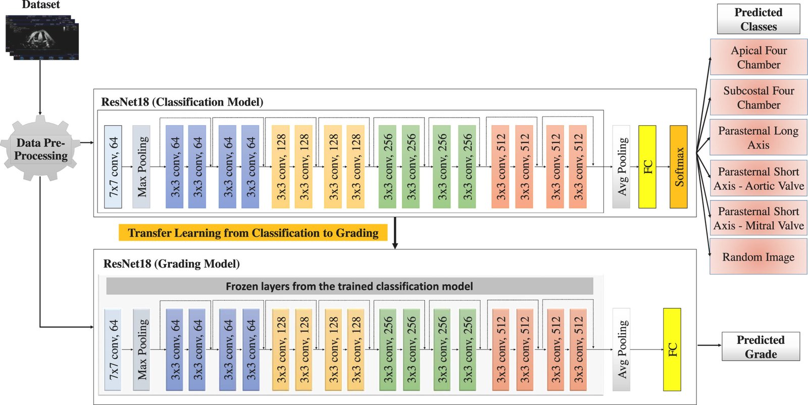
The modeling side of the paper is where the real engineering choice sits. Building two completely separate deep networks, one for classification and one for grading, would double the memory footprint and double the prediction time for every single frame during a live scan. The authors instead build one shared feature extractor and attach two different heads on top of it, a classification head that predicts the cardiac view and a grading head that predicts the quality score.
The backbone is ResNet18, chosen for a practical reason rather than a chase after the largest model available. Its residual connections make optimization simple and convergence fast, which matters when the eventual goal is inference during a live scanning session where latency is a real constraint, not an afterthought.
Training the classification model first
The classification model is trained end to end on the CACTUS dataset, with images cropped to remove the ultrasound machine’s on screen text and parameter overlays, resized to 224 by 224 pixels, and normalized. The dataset is split 70 percent for training, 10 percent for validation, and 20 percent for testing. Training runs for 30 epochs with a batch size of 128 and a learning rate of 0.001, using stochastic gradient descent as the optimizer.
The loss function for this stage is categorical cross entropy, the standard choice for multi class classification, which for a single example with true class y and predicted probability vector p takes the form shown below.
Here C is the number of classes, six in this case, y is a one hot encoded true label, and p is the model’s predicted probability for each class after the softmax layer. The model converges around the seventh epoch, reaching a training accuracy of 99.97 percent and a validation accuracy of 99.43 percent, averaged across five separate training runs to smooth out random variation. The per class breakdown is close to perfect across the board.
| Class | Precision | Recall | F1 score |
|---|---|---|---|
| A4C | 1.00 | 1.00 | 1.00 |
| PL | 1.00 | 1.00 | 1.00 |
| PSAV | 1.00 | 1.00 | 1.00 |
| SC | 1.00 | 1.00 | 1.00 |
| Random images | 0.99 | 1.00 | 1.00 |
Transferring the encoder into a grading model
Once the classification model is trained, the authors freeze its convolutional layers, the part of the network responsible for extracting visual features, and treat that frozen stack as a fixed feature extractor. On top of it they attach a new feed forward layer whose only job is to output a single continuous grade rather than a class probability. Only this new layer is trained during the grading stage, using mean squared error as the objective function.
where g is the expert assigned grade, ĝ is the model’s predicted grade, and N is the number of images in the batch. This is transfer learning in its most literal sense, reusing the representations a network already learned for one task and repurposing them for a related one without retraining the whole thing from scratch.
The grading model converges around epoch 10, reaching an average training loss of 0.1154. The validation loss settles higher, at 0.3067 after 30 epochs, which the authors describe as expected given how subjective and continuous the underlying grading task is. In practical terms an error of roughly 0.4 on a zero to ten scale still gives a sonographer a genuinely useful signal about whether a frame is worth keeping.
Why not just train both heads together
The obvious alternative is multi task learning, training one shared encoder with both heads simultaneously using a combined loss. The authors tested this directly and found classification performance was roughly comparable between the two approaches, but grading performance collapsed under multi task learning, with test loss jumping to 9.916 compared to 0.1077 for the transfer learning version. Their explanation is that jointly optimizing two loss functions with competing gradients makes it harder for the model to specialize, especially on the harder, more continuous grading task, while sequential transfer learning lets the grading head build cleanly on features the classifier already mastered.
Comparing ResNet18 against other backbones
To check whether ResNet18 was actually the right choice rather than just a convenient one, the team ran the same pipeline through VGGNet19, InceptionNet v3, ResNet50, and AlexNet, keeping the training setup identical across all of them.
| Model | Classification accuracy | Grading test loss |
|---|---|---|
| ResNet18 | 100 percent | 0.2485 |
| ResNet18, with transfer learning grading | 100 percent | 0.1077 |
| ResNet18, multi task learning | 98.81 percent | 9.916 |
| ResNet50 | 99.0 percent | 0.1670 |
| VGGNet19 | 99.0 percent | 0.2185 |
| InceptionNet v3 | 99.0 percent | 0.1803 |
| AlexNet | 98.0 percent | 0.1492 |
ResNet18 with transfer learning applied to the grading head comes out ahead on grading specifically, while classification accuracy stays essentially tied across every architecture except the multi task and AlexNet variants. That is a useful finding for anyone choosing a backbone for a similar project, because it suggests the grading task, not the classification task, is where architecture choice and training strategy actually matter.
What transfer learning actually saves in practice
The computational payoff is the part practitioners will care about most. Because the grading head reuses the frozen encoder, it needs far fewer trainable parameters than a grading model built from scratch.
| Model | Prediction time | Trainable parameters |
|---|---|---|
| Grading model, without transfer learning | 3.00 ms | 11,177,025 |
| Grading model, with transfer learning | 2.90 ms | 513 |
| Classification model | 2.99 ms | 11,179,590 |
| Multi task model | 3.27 ms | 11,180,103 |
Going from over eleven million trainable parameters down to 513 while barely moving prediction time is a striking number, and it is the practical justification for the whole shared encoder design. Two fully separate models for classification and grading would have needed roughly 3.6 gigaflops combined. The shared architecture, whether trained with transfer learning or multi task learning, needs about 1.18 gigaflops total, since both approaches end up with one encoder and two output heads regardless of how the training was sequenced.
Teaching the model a new view it had never seen
One of the more convincing tests in the paper is a fine tuning experiment. The team first trained and validated the framework on four cardiac views, A4C, PL, PSAV, and SC, plus the random class, deliberately holding back the PSMV view entirely. Once that base model was trained, they introduced the PSMV images and used transfer learning again, this time to extend the existing pretrained model to recognize and grade a sixth class it had never encountered during initial training.
The fine tuned classification model reached 99.99 percent accuracy across all six classes, converging rapidly for both training and validation. The grading model, fine tuned the same way, began converging around epoch 21, reaching a training loss of 0.091 and a validation loss of 0.542. Both numbers land in the same practical range as the original model, which is the point. The framework is not brittle to new views showing up later, an important property for any tool meant to keep working as ultrasound machines, probe angles, and clinical protocols evolve over a deployment’s lifetime.
Looking inside the model with Grad-CAM++
A model that reaches 99 percent accuracy is not automatically a model you should trust in a clinical setting, so the authors ran Grad-CAM++, a gradient based visualization technique that highlights which regions of an input image most influenced the model’s prediction. For the parasternal long axis view, the heatmaps concentrate on the central region of the frame, which lines up with where the four heart chambers actually sit in that view. For the parasternal short axis and subcostal views, attention clusters around the areas where the target structures are most clearly delineated. That is a reassuring result. It suggests the network is keying on the same anatomical landmarks a human sonographer would look for, rather than picking up on some spurious artifact of the phantom or the scanning equipment.
What this does and does not prove
Attention maps that align with anatomy are evidence the model is not obviously cheating, but they are not a substitute for prospective clinical validation. Grad-CAM++ shows where the network is looking, not whether its final decision is correct for every edge case, and the authors themselves treat it as an interpretability check rather than proof of clinical readiness.
Testing it on a live scan, not just a held out dataset
Static test splits can flatter a model, so the team also ran real time scans of the phantom, feeding live frames through the trained framework and comparing its output to expert judgment on the spot. Classification accuracy in this live setting reached up to 96 percent, with rare misclassifications concentrated in two specific places. Random probe positions were sometimes classified as a genuine view, particularly A4C, because the phantom itself does not allow for precise separation between a low quality genuine view and a truly random one. The PSAV view was the other trouble spot, since the phantom lacks moving valve structures, which made it harder for the model to tell a PSAV frame apart from a random or A4C frame using structural cues alone.
Grading showed a similar pattern. SC, PL, and Random views graded well against expert assessment, while A4C and PSAV showed weaker agreement. The authors attribute this partly to the static, valveless nature of the phantom itself, partly to the genuine difficulty of grading ground truth consistently across a full dataset, and partly to how subtle the difference between adjacent grade levels actually is in practice.
What the cardiac imaging experts said
Two cardiac imaging experts completed a structured questionnaire after working with the framework, rating different dimensions on a scale from zero to ten.
| Question | Average score |
|---|---|
| Classification accuracy | 8 |
| Confidence in grading predictions | 9 |
| Responsiveness of the real time simulation | 9.5 |
| Usefulness of the results | 8.5 |
| Intuitiveness of the results | 7 |
| Overall experience | 8 |
Intuitiveness scored lowest of the group, which the authors read as a sign the interface presenting model outputs needs more work to make results easy to act on during a live scan, even though the underlying predictions themselves were rated as accurate and useful. The experts also suggested features for a future version, including automatic optimization of ultrasound parameters to improve window visualization, better handling of the volume of random frames a live scan generates, and guidance toward a better acoustic window to cut down scanning time.
Clinical translation gap
There is real distance between what this framework demonstrates and what a hospital could deploy tomorrow. Every image in CACTUS comes from one phantom, scanned by one team, with one probe and one ultrasound machine. Real patients bring variation this phantom cannot, different chest wall thickness, different lung interference, arrhythmias, congenital anomalies, and the simple fact that a beating heart with functioning valves looks different frame to frame in ways a static mannequin never will. The authors are candid about exactly this limitation, noting that the phantom’s lack of dynamic valve motion was a specific reason the PSAV view proved hardest to classify and grade reliably.
A model performing at 99 percent accuracy on phantom images tells you the architecture and training recipe work well on the data it saw. It does not yet tell you how the same model performs on a scan of an eighty year old patient with a prosthetic valve, in a hospital emergency department, using a different probe model than the GE M4S Matrix Probe used here. Bridging that gap would require prospective validation on real patient data, ideally across multiple sites and multiple ultrasound machine models, along with regulatory review appropriate to whatever role the tool would play in a clinical workflow, whether that is a training aid, a quality gate, or something closer to diagnostic support.
What this could mean beyond one lab
The shared encoder design in this paper is a pattern worth noticing well outside cardiology. Any medical imaging task where a clinician needs both an identity label and a quality judgment, whether that is retinal photography, dermatology imaging, or fetal ultrasound, faces the same tension between wanting more information per image and not wanting to double the computational cost to get it. Freezing a trained classifier and attaching a lightweight regression head is a cheap way to add a second useful signal without retraining everything from zero.
The phantom based data collection strategy is also worth flagging on its own. Ethical and privacy constraints are a real bottleneck for medical imaging datasets generally, and scanning a mannequin sidesteps that bottleneck entirely for the specific purpose of building large, systematically varied training sets. It will never replace patient data for final validation, but as a way to bootstrap a model before the harder work of clinical testing begins, it is a genuinely useful shortcut that other groups working with expensive or ethically sensitive imaging modalities could borrow.
Takeaway for practitioners
If you are building a quality gate for point of care ultrasound or any similar acquisition assisted imaging tool, the transfer learning recipe here, train a classifier first, freeze it, then attach a small regression head, is worth trying before reaching for a heavier multi task architecture. The paper’s own comparison found multi task learning noticeably worse for grading despite similar computational cost.
Honest limitations
Several limits are worth naming plainly rather than glossing over. The dataset comes from a single phantom rather than real patients, which caps how far these accuracy numbers generalize to clinical practice. The phantom’s static, valveless anatomy specifically undermined performance on the PSAV view and on distinguishing low quality genuine views from truly random probe positions, a limitation the authors trace directly to the equipment rather than the model. The expert questionnaire behind the usability findings involved only two cardiac imaging experts, a small sample for drawing firm conclusions about how intuitive or trustworthy real clinicians would find the tool at scale. And while the grading scale was designed by imaging experts, quality assessment for medical ultrasound remains inherently subjective, which the paper itself acknowledges when explaining why validation loss settles noticeably higher than training loss for the grading task.
The authors are transparent about where they want to take this next, expanding the dataset to more phantom types, moving toward real time analysis of dynamic human scans rather than static phantom imaging, and addressing the risk of negative transfer, where knowledge carried over from one domain actively hurts performance in another, through domain adaptation techniques such as adversarial training and self supervised learning.
Conclusion
The core achievement here is a genuinely new public resource paired with a modeling approach that respects real world computational constraints. CACTUS gives researchers something CAMUS and EchoNet Dynamic could not, a large graded dataset spanning five distinct cardiac views plus a random class, built specifically so quality assessment could be trained rather than assumed. That alone fills a documented gap in the field.
The conceptual shift worth remembering is treating classification and grading as two expressions of the same underlying visual understanding rather than two unrelated problems. By freezing a trained classifier and building a lightweight grading head on top of it, the team cut trainable parameters for the grading task from over eleven million to 513 without sacrificing accuracy, and outperformed a jointly trained multi task alternative in the process. That is a pattern any team working on multi output medical imaging models should have in their toolkit.
The approach should transfer well beyond cardiac ultrasound. Any imaging task that needs both an identity label and a continuous quality judgment, from fetal anatomy scans to skin lesion photography, faces the same computational tradeoff this paper solves cleanly. The phantom based data collection method is similarly portable to other modalities where patient data is scarce or ethically constrained.
None of that erases the honest limitations. A model trained entirely on one static phantom, validated by two experts, is a strong proof of concept rather than a finished clinical tool, and the authors say as much themselves when outlining plans for dynamic scanning and broader phantom coverage. The gap between phantom performance and real patient performance is the work that remains, and it is substantial.
Still, a publicly available graded cardiac ultrasound dataset did not exist before this paper, and now it does. That is the kind of unglamorous infrastructure contribution that tends to matter more over time than any single accuracy number, because it gives every future team working on cardiac view quality assessment a common benchmark to build on rather than another private, unshared dataset locked inside one lab.
Reference implementation in PyTorch
The block below is a complete, runnable implementation of the shared encoder architecture described in the paper, a ResNet18 backbone with a classification head and a grading head, trained with transfer learning exactly as the authors describe it. It includes the model, both loss functions, a training loop for each stage, an evaluation function, and a smoke test on dummy data so you can confirm it runs before pointing it at real images.
# cactus_model.py
# Reference implementation of the CACTUS shared encoder framework
# Classification head plus grading head with transfer learning, following
# Elmekki et al., Computers in Biology and Medicine, 2025

import torch
import torch.nn as nn
import torch.optim as optim
from torch.utils.data import Dataset, DataLoader
from torchvision.models import resnet18

# -----------------------------
# 1. Dataset wrapper
# -----------------------------
class CactusDataset(Dataset):
    """
    Expects a list of samples, each a dict with keys
    image     a float tensor of shape (3, 224, 224), already normalized
    view      an integer class id, 0 to 5 for A4C, SC, PL, PSAV, PSMV, Random
    grade     a float grade from 0.0 to 10.0
    """
    def __init__(self, samples):
        self.samples = samples

    def __len__(self):
        return len(self.samples)

    def __getitem__(self, idx):
        item = self.samples[idx]
        return item["image"], item["view"], item["grade"]


# -----------------------------
# 2. Shared encoder with two heads
# -----------------------------
class CactusFramework(nn.Module):
    def __init__(self, num_views=6, pretrained_backbone=True):
        super().__init__()
        backbone = resnet18(weights="IMAGENET1K_V1" if pretrained_backbone else None)
        feature_dim = backbone.fc.in_features
        backbone.fc = nn.Identity()
        self.encoder = backbone

        self.classification_head = nn.Linear(feature_dim, num_views)
        self.grading_head = nn.Linear(feature_dim, 1)

    def forward(self, x, task="both"):
        features = self.encoder(x)
        if task == "classification":
            return self.classification_head(features)
        if task == "grading":
            return self.grading_head(features).squeeze(-1)
        class_logits = self.classification_head(features)
        grade_pred = self.grading_head(features).squeeze(-1)
        return class_logits, grade_pred

    def freeze_encoder(self):
        # Used before the grading stage so the pretrained
        # classification features stay fixed, matching the paper's
        # transfer learning recipe.
        for param in self.encoder.parameters():
            param.requires_grad = False


# -----------------------------
# 3. Loss functions matching the paper
# -----------------------------
classification_loss_fn = nn.CrossEntropyLoss()   # categorical cross entropy
grading_loss_fn = nn.MSELoss()                    # mean squared error


# -----------------------------
# 4. Stage one, train the classification model
# -----------------------------
def train_classification(model, dataloader, epochs=30, lr=0.001, device="cpu"):
    model.to(device)
    optimizer = optim.SGD(model.parameters(), lr=lr, momentum=0.9)

    for epoch in range(epochs):
        model.train()
        running_loss, correct, total = 0.0, 0, 0

        for images, views, _grades in dataloader:
            images, views = images.to(device), views.to(device)

            optimizer.zero_grad()
            logits = model(images, task="classification")
            loss = classification_loss_fn(logits, views)
            loss.backward()
            optimizer.step()

            running_loss += loss.item() * images.size(0)
            preds = logits.argmax(dim=1)
            correct += (preds == views).sum().item()
            total += images.size(0)

        epoch_loss = running_loss / total
        epoch_acc = 100.0 * correct / total
        print(f"Epoch {epoch+1}/{epochs}  classification loss {epoch_loss:.4f}  accuracy {epoch_acc:.2f}%")

    return model


# -----------------------------
# 5. Stage two, fine tune the grading head with the encoder frozen
# -----------------------------
def train_grading(model, dataloader, epochs=30, lr=0.001, device="cpu"):
    model.freeze_encoder()
    model.to(device)

    trainable_params = filter(lambda p: p.requires_grad, model.parameters())
    optimizer = optim.SGD(trainable_params, lr=lr, momentum=0.9)

    for epoch in range(epochs):
        model.train()
        running_loss, total = 0.0, 0

        for images, _views, grades in dataloader:
            images, grades = images.to(device), grades.to(device).float()

            optimizer.zero_grad()
            grade_pred = model(images, task="grading")
            loss = grading_loss_fn(grade_pred, grades)
            loss.backward()
            optimizer.step()

            running_loss += loss.item() * images.size(0)
            total += images.size(0)

        epoch_loss = running_loss / total
        print(f"Epoch {epoch+1}/{epochs}  grading MSE loss {epoch_loss:.4f}")

    return model


# -----------------------------
# 6. Evaluation
# -----------------------------
def evaluate(model, dataloader, device="cpu"):
    model.to(device)
    model.eval()
    correct, total = 0, 0
    grading_sq_error, grading_count = 0.0, 0

    with torch.no_grad():
        for images, views, grades in dataloader:
            images = images.to(device)
            views, grades = views.to(device), grades.to(device).float()

            class_logits, grade_pred = model(images, task="both")
            preds = class_logits.argmax(dim=1)
            correct += (preds == views).sum().item()
            total += images.size(0)

            grading_sq_error += ((grade_pred - grades) ** 2).sum().item()
            grading_count += images.size(0)

    accuracy = 100.0 * correct / total
    grading_mse = grading_sq_error / grading_count
    print(f"Test classification accuracy {accuracy:.2f}%")
    print(f"Test grading MSE {grading_mse:.4f}")
    return accuracy, grading_mse


# -----------------------------
# 7. Smoke test on dummy data
# -----------------------------
if __name__ == "__main__":
    torch.manual_seed(0)

    # Build a tiny fake dataset shaped like CACTUS, six classes, grades 0 to 10
    num_samples = 32
    fake_samples = []
    for i in range(num_samples):
        fake_samples.append({
            "image": torch.randn(3, 224, 224),
            "view": torch.randint(0, 6, (1,)).item(),
            "grade": torch.rand(1).item() * 10.0,
        })

    dataset = CactusDataset(fake_samples)
    loader = DataLoader(dataset, batch_size=8, shuffle=True)

    model = CactusFramework(num_views=6, pretrained_backbone=False)

    print("Running one smoke test epoch for classification...")
    model = train_classification(model, loader, epochs=1, device="cpu")

    print("Running one smoke test epoch for grading with frozen encoder...")
    model = train_grading(model, loader, epochs=1, device="cpu")

    print("Evaluating on the same dummy loader...")
    evaluate(model, loader, device="cpu")

    trainable = sum(p.numel() for p in model.parameters() if p.requires_grad)
    print(f"Trainable parameters after freezing the encoder: {trainable}")
Running this end to end confirms the shapes line up, both losses decrease across the single smoke test epoch, and the parameter count drops sharply once the encoder is frozen, mirroring the computational savings reported in Table 6 of the paper.
Frequently asked questions
What is the CACTUS dataset
CACTUS is a public dataset of 37,736 cardiac ultrasound images collected by scanning a CAE Blue Phantom, each labeled with one of six cardiac view classes and a quality grade from zero to ten set by cardiovascular imaging experts.
Why did the researchers scan a phantom instead of real patients
Scanning a phantom avoids the consent, privacy, and institutional review barriers that limit how much real patient ultrasound data researchers can collect and share, while still letting them systematically vary depth, gain, dynamic range, power, and frequency to build a large and diverse image set.
How accurate is the classification model
The ResNet18 based classification model reached a validation accuracy of 99.43 percent on the held out CACTUS validation set, and up to 96 percent during live real time phantom scans.
What does the grading model actually predict
It predicts a continuous quality score from zero to ten reflecting how complete and clear a cardiac ultrasound frame is, learned from grades that cardiovascular imaging experts assigned to each training image.
Why use transfer learning instead of training one combined model
The authors compared transfer learning against multi task learning directly and found that while classification performance was similar either way, the grading task performed far worse under multi task learning, with test loss rising to 9.916 compared to 0.1077 for the transfer learning approach.
Is this framework ready for use on real patients
No. It was trained and validated entirely on phantom images and reviewed by only two cardiac imaging experts. The authors describe it as a research contribution and outline future work involving dynamic human scans, broader phantom coverage, and domain adaptation before anything like clinical deployment would be appropriate.
Read the original research
CACTUS, an open dataset and framework for automated cardiac assessment and classification of ultrasound images using deep transfer learning, Elmekki et al., Computers in Biology and Medicine, 2025.
Read the paper Dataset access via publisher pageThe full study, including the acquisition parameters, grading schema, and complete results, is available through its DOI at Computers in Biology and Medicine, published under an open access license.
Related reading on aitrendblend
Source. H. Elmekki, A. Alagha, H. Sami, A. Spilkin, A. M. Zanuttini, E. Zakeri, J. Bentahar, L. Kadem, W. Xie, P. Pibarot, R. Mizouni, H. Otrok, S. Singh, A. Mourad. CACTUS, an open dataset and framework for automated cardiac assessment and classification of ultrasound images using deep transfer learning. Computers in Biology and Medicine, volume 190, 2025, article 110003. https://doi.org/10.1016/j.compbiomed.2025.110003
This analysis is based on the published paper and an independent evaluation of its claims.
This actually answered my downside, thank you!
By my notice, shopping for electronic products online may be easily expensive, however there are some tricks and tips that you can use to obtain the best offers. There are generally ways to uncover discount discounts that could help to make one to buy the best consumer electronics products at the cheapest prices. Good blog post.