
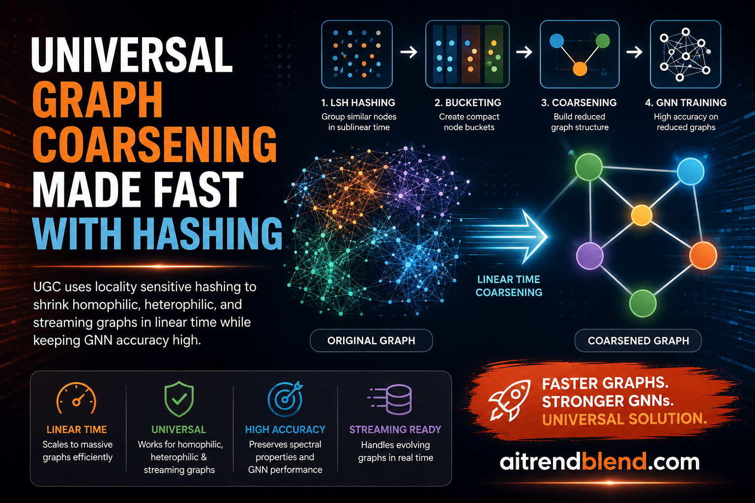
Imagine a citation graph with more than seven hundred thousand papers, each carrying a bag of words feature vector and a web of references to its neighbors. Training a graph neural network on something that size can exhaust memory before it finishes a single epoch. A team at the Indian Institute of Technology Delhi asks a blunt question. What if you could squeeze that graph down to a fraction of its size in linear time, keep both the wiring and the node attributes intact, and do it without ever solving an expensive optimization problem?
Key points
- UGC is a graph coarsening method that groups similar nodes into supernodes using locality sensitive hashing, so it runs in time that grows only with the number of nodes plus edges.
- It builds an augmented feature for every node by blending node attributes with the adjacency vector, weighted by a heterophily factor, which lets one method serve both homophilic and heterophilic graphs.
- On the Physics dataset it reached a 50 percent coarsening roughly six times faster than Kron reduction, and on Squirrel it ran about nine times faster than algebraic distance.
- A streaming variant updates the coarsened graph as new nodes arrive, with cost tied only to the new data rather than the whole graph.
- Graph neural networks trained on the coarsened graphs held or improved node classification accuracy on nine of eleven datasets.
- The work appeared in IEEE Transactions on Pattern Analysis and Machine Intelligence in 2026, extending an earlier NeurIPS 2024 paper, with public code on GitHub.
Why shrinking a graph is harder than it sounds
Graphs keep getting bigger. Social networks, transport maps, protein interaction networks, and citation graphs now reach into the hundreds of millions of nodes. The standard trick for taming them is coarsening, which replaces a large graph with a smaller one that behaves almost the same way. Instead of solving your problem on the full graph, you solve a lookalike at a lower cost and lift the answer back up.
The problem runs deeper than it first appears. Most coarsening methods only look at structure. They study who connects to whom and ignore what each node actually contains. That works until you remember that real nodes carry context. A person in a social graph has an age and a location. A protein has a measured quantity. A paper has a topic. Throw that away during coarsening and the smaller graph loses the very information you wanted to keep.
The methods that do fold in node features tend to be slow. Optimization based approaches from Loukas and from Kumar give strong similarity guarantees, yet they lean on nonconvex problems that eat compute and stall on large graphs. Graph condensation methods such as GCond go further and match gradients between a synthesized small graph and the original, which means training a full network just to build the smaller one. That is a heavy price for a preprocessing step.
There is a second blind spot. Most methods assume homophily, the tendency of similar nodes to connect. Citation networks fit that pattern because papers cite others in the same field. Plenty of important graphs do not. In a financial fraud network, a normal account often links to a suspicious one, so neighbors are deliberately dissimilar. That is heterophily, and coarsening methods built for homophily quietly break on it.
And almost none of the classic methods handle change well. When a graph grows one node at a time, as a live social feed or a stream of transactions does, the usual answer is to recompute the whole coarsened graph from scratch at every step. For a graph that never stops moving, that is a losing race.
The core idea behind UGC
UGC stands for Universal Graph Coarsening. The word universal is doing real work here. The authors, Mohit Kataria, Nikita Malik, Jayadeva, and Sandeep Kumar, wanted one method that copes with homophilic graphs, heterophilic graphs, and streaming graphs without changing its machinery. The route they take is hashing rather than optimization, and that single choice explains most of the speed.
The first move is to stop treating structure and features as separate. For every node UGC builds an augmented feature that stitches the node attributes together with the node adjacency vector. A tuning knob called the heterophily factor, written as alpha and living between zero and one, decides how much weight each part gets. When a graph is strongly homophilic the attributes carry most of the signal. When it leans heterophilic the wiring matters more. The augmented feature for a node combines both.
Here \(X_i\) is the attribute vector, \(A_i\) is the row of the adjacency matrix for node i, and the double bar is concatenation. The heterophily factor alpha is computed once as the fraction of edges that link nodes of different classes, so the data itself sets the balance rather than a human guessing.
The second move is where the speed comes from. UGC hashes these augmented features with locality sensitive hashing, a family of functions built so that vectors close together in space are likely to land in the same bucket, while distant vectors rarely do. Each hash function is a random projection drawn from a stable distribution, followed by a floor operation that drops the projected value into a fixed width bin.
The matrix \(W\) holds the random projectors and \(b\) is a random bias, both sampled from a 2-stable distribution. The number \(r\) is the bin width, the one hyperparameter that controls how aggressive the coarsening gets. A wider bin drops more nodes into each bucket and yields a smaller graph. UGC runs several projectors and, for each node, keeps the bin index that shows up most often across them. Nodes that share that winning index get merged into one supernode.
Once the assignment is fixed, UGC records it in a loading matrix \(C\) where each row has exactly one nonzero entry marking which supernode a node joins. Building the coarsened graph from there is direct matrix algebra. The coarsened adjacency and the supernode features fall out of the loading matrix and the originals.
Every edge in the small graph pools the edges that ran between the merged groups, so the coarsened adjacency is far sparser than the original. The three phases together, building the augmented matrix, hashing into bins, and reading off the supernode edges, add up to a cost that grows with the number of nodes plus the number of edges. That linear behavior is what the authors mean when they call UGC fast.
Keeping the graph faithful
Speed would be worthless if the coarsened graph forgot what the original looked like. UGC leans on a similarity measure called epsilon similarity, which compares the Laplacian norms of the feature matrices before and after coarsening. If the two norms stay close, the smaller graph preserves the smoothness of the node features across edges.
The paper proves that the basic UGC output is epsilon similar with epsilon at least zero. That is a guarantee, but a loose one. To tighten it the authors add an optional stage called UGC with feature relearning. Rather than averaging the features of merged nodes, this stage solves a small convex problem that enforces smoothness on the supernode features, and it has a clean closed form solution.
With relearned features the bound tightens so that epsilon sits between zero and one, which is the range that matters for practical use. The nice part is that this remains a closed form step rather than an iterative grind, so it does not throw away the speed advantage. A reader who wants the full proofs will find them in the supplementary material of the published IEEE TPAMI paper, which also carries the theorem on hash collision probability.
That collision theorem is worth pausing on. It states that the chance two nodes end up in the same supernode falls as the distance between their augmented features grows. The team checked this directly by measuring feature distances on Cora and Citeseer and counting how often close pairs really did share a supernode. The empirical curve matched the theory, which is the sort of small validation that separates a claim you can trust from one you cannot.
How fast is fast
The runtime story is the heart of the paper, and the numbers are concrete. On the Physics dataset, which has about 34 thousand nodes and 247 thousand edges, UGC reached a 50 percent coarsening roughly six times faster than Kron reduction. On the Squirrel dataset, near 5 thousand nodes and 217 thousand edges, it ran about nine times faster than the algebraic distance method. Those are not marginal gains.
| Dataset | Approx nodes | What UGC did |
|---|---|---|
| Physics | 34,000 | Coarsened about six times faster than Kron reduction |
| Squirrel | 5,000 | Coarsened about nine times faster than algebraic distance |
| Roughly seven times Physics | Coarsened in about one third the time the fastest rivals needed on Physics | |
| Yelp | 716,847 | Coarsened at a scale existing methods could not reach |
The Reddit result deserves a second look. Reddit carries roughly seven times as many nodes as Physics, and UGC coarsened it in about a third of the time the fastest competing methods took on the much smaller Physics graph. Yelp, at more than seven hundred thousand nodes, simply was not reachable by the older methods at all. UGC handled it. When the authors add that eigenvalue error checks ran out of memory on these giants while rival methods failed to produce any coarsened graph, the contrast is stark.
UGC can coarsen down massive datasets like Yelp, which has 716,847 nodes, which was previously not possible. Kataria and colleagues, IEEE TPAMI 2026
There is a subtlety in how the team reports these times, and it is worth flagging because it is honest. The bin width has to be tuned once per dataset with a small binary search, and that tuning cost sits outside the reported runtime. The authors say so plainly rather than folding it into the headline number. It is a one time cost per dataset, but a reader planning a deployment should budget for it.
Where the augmented feature earns its keep
The clearest evidence that blending features with structure matters shows up on heterophilic graphs. The team compares two settings, one where hashing uses features alone and one where it uses the augmented feature that adds the adjacency vector. On homophilic graphs the eigen error results land in the same neighborhood as existing methods, competitive but not dramatic. On heterophilic datasets the augmented version pulls clearly ahead.
That gap tells the real story. A method that only hashed raw features would behave like every other homophily leaning tool and stumble when neighbors are dissimilar. By folding the wiring into the hash, UGC keeps working when the graph refuses to be homophilic. The authors call this the true potential of the approach, and the eigen error tables back the phrase with data rather than adjectives.
They also ran a neat ablation on the heterophily factor itself. Setting alpha close to the measured heterophily factor of a dataset gave the best results across both heterophilic graphs like Squirrel and Chameleon and homophilic ones like Cora and Pubmed. In other words the parameter has a natural setting that the data hands you, rather than a knob you have to sweep blindly.
The streaming extension
Static graphs are a convenient fiction. Real networks grow. UGC Stream is the extension that handles this, and it is arguably the most practical contribution. When new nodes arrive at a timestamp, the method does not rebuild the coarsened graph. It only maps the new nodes and their affected neighbors into supernodes and patches the loading matrix.
The cost of each update tracks only the number of new nodes and new edges, not the accumulated size of the whole graph. The paper writes this incremental complexity as \(O(\lvert \Delta V_\tau \rvert + \lvert \Delta E_\tau \rvert)\), which for a slow growing graph is a rounding error next to a full recomputation. The authors describe three update modes, from fixed supernode assignments where old nodes never move, to dynamic assignments that let existing nodes switch supernodes, to a mode that spawns brand new supernodes as the structure shifts.
To test it they split each dataset into training, validation, and test portions weighted at 60, 20, and 20 percent, then fed the training data in as a stream. The first 20 percent arrived at the start and the rest came in 10 percent increments. A network trained on the incrementally coarsened stream reached the same node classification accuracy as a network trained on the full dataset coarsened all at once. Matching the batch result while paying only incremental cost is the outcome you want from a streaming method.
Does the coarsened graph still work for learning
A coarsened graph is only useful if you can train on it and still make good predictions on the original. The team tested this with graph convolutional networks, using a modest single hidden layer of sixteen neurons. The recipe is simple. Coarsen the graph, train the network on the small version, then use the learned weights to predict on the full graph.
Across eleven datasets, networks trained on UGC coarsened graphs held or improved node classification accuracy on nine of them. Even at a 70 percent coarsening ratio, where the graph shrinks to less than a third of its nodes, accuracy on most datasets held up. On heterophilic graphs, where the augmented feature shines, the combined feature and adjacency version delivered the largest accuracy gains, in some cases beating the accuracy of a network trained on the whole uncoarsened dataset.
The method is not tied to one architecture either. The authors repeated the test with GraphSAGE, GIN, and GAT and saw the pattern hold, which tells you the coarsened graph preserves something general about the data rather than something a single model happens to exploit. They also pushed beyond node classification to link prediction, training a link prediction network on the coarsened graph and asking it to recover held out edges of the original. It stayed competitive across homophilic and heterophilic benchmarks, evidence that the coarsening keeps edge level structure and not just node level labels.
The honest limitations
No method is free, and the paper is refreshingly candid about the tradeoffs. The bin width tuning is the first. It has to be found per dataset with a binary search, and although the authors provide an efficient routine for it, the cost is real and sits outside the reported runtime. A team adopting UGC should treat that search as part of the setup budget.
The second is the tension between coarsening ratio and fidelity. Push the ratio higher and the relative eigen error grows, meaning the spectral approximation loosens. The authors show accuracy holds well up to moderate ratios and then slips as you compress harder. There is no magic here. Smaller graphs carry less information, and beyond some point that shows up in results. The right ratio is a judgment call tied to how much accuracy a task can spare.
Third, the relative eigen error itself is an imperfect guide. The paper points out that on the PubMed dataset UGC did not always post the best eigen error yet still delivered the strongest downstream accuracy. That mismatch is a useful caution. A single spectral metric does not fully predict how a coarsened graph will perform on a real task, and the authors say more investigation is needed on the link between eigen error and downstream results. Treating the eigen error as the last word would be a mistake.
Finally, the default hashing uses randomized projectors for speed. The authors note you could swap in learned hash functions tuned to a dataset, which might improve grouping, but that adds the overhead of training an auxiliary model and chips away at the speed that is the whole point. They frame learned hashing as an optional plug in for when extra compute is acceptable rather than a default, which is the sensible read.
A reference implementation in PyTorch
The paper ships public code, and the pipeline is compact enough to sketch end to end. The implementation below builds the augmented feature, hashes it with random stable projectors, forms the loading matrix by majority bin voting, and constructs the coarsened adjacency and features. It also includes the feature relearning step and an epsilon similarity check, with a runnable smoke test on a small random graph. The official repository lives on the author GitHub page for UGC.
# Universal Graph Coarsening (UGC) reference implementation
# Hashing based coarsening with optional feature relearning.
import torch
import torch.nn as nn


def heterophily_factor(edge_index, labels):
    # Fraction of edges that join nodes of different classes.
    src, dst = edge_index
    diff = (labels[src] != labels[dst]).float()
    return diff.mean().item()


def build_augmented_features(X, A, alpha):
    # F_i = concat((1 - alpha) * X_i, alpha * A_i)
    return torch.cat([(1.0 - alpha) * X, alpha * A], dim=1)


class UGC(nn.Module):
    def __init__(self, in_dim, num_projectors=64, bin_width=1.0, seed=0):
        super().__init__()
        g = torch.Generator().manual_seed(seed)
        # Projectors and bias drawn from a 2-stable (normal) distribution.
        self.W = torch.randn(in_dim, num_projectors, generator=g)
        self.b = torch.rand(num_projectors, generator=g)
        self.r = bin_width

    def hash_indices(self, F):
        # One integer bin per node per projector.
        proj = (F @ self.W + self.b) / self.r
        return torch.floor(proj).long()          # shape [N, num_projectors]

    def assign_supernodes(self, H):
        # For each node keep the bin index that appears most across projectors,
        # then relabel the surviving codes to contiguous supernode ids.
        N = H.shape[0]
        codes = torch.zeros(N, dtype=torch.long)
        for i in range(N):
            vals, counts = torch.unique(H[i], return_counts=True)
            codes[i] = vals[torch.argmax(counts)]
        uniq, pi = torch.unique(codes, return_inverse=True)
        return pi, uniq.numel()                   # pi in [0, n), n supernodes

    def loading_matrix(self, pi, n):
        # C[v, pi[v]] = 1, one nonzero per row.
        N = pi.shape[0]
        C = torch.zeros(N, n)
        C[torch.arange(N), pi] = 1.0
        return C

    def forward(self, X, A, alpha):
        F = build_augmented_features(X, A, alpha)
        H = self.hash_indices(F)
        pi, n = self.assign_supernodes(H)
        C = self.loading_matrix(pi, n)
        A_coarse = C.t() @ A @ C                 # A' = C^T A C
        # Supernode features as the mean of member node features.
        counts = C.sum(dim=0).clamp(min=1.0).unsqueeze(1)
        F_coarse = (C.t() @ F) / counts
        return A_coarse, F_coarse, C, pi, n


def laplacian(A):
    D = torch.diag(A.sum(dim=1))
    return D - A


def relearn_features(C, L, F, alpha):
    # Closed form: F'' = (2/alpha * C^T L C + C^T C)^-1 C^T F
    lhs = (2.0 / alpha) * (C.t() @ L @ C) + (C.t() @ C)
    rhs = C.t() @ F
    return torch.linalg.solve(lhs, rhs)


def laplacian_norm(F, L):
    # sqrt(trace(F^T L F)), the Laplacian norm used in epsilon similarity.
    return torch.sqrt(torch.trace(F.t() @ L @ F).clamp(min=0.0))


def smoke_test():
    torch.manual_seed(0)
    N, d = 200, 16
    # Random symmetric adjacency with no self loops.
    rand = (torch.rand(N, N) < 0.05).float()
    A = torch.triu(rand, diagonal=1)
    A = A + A.t()
    X = torch.randn(N, d)
    labels = torch.randint(0, 4, (N,))
    edge_index = A.nonzero().t()
    alpha = max(heterophily_factor(edge_index, labels), 1e-3)

    model = UGC(in_dim=d + N, num_projectors=64, bin_width=2.0)
    A_c, F_c, C, pi, n = model(X, A, alpha)

    L = laplacian(A)
    L_c = laplacian(A_c)
    F_aug = build_augmented_features(X, A, alpha)
    F_relearned = relearn_features(C, L, F_aug, alpha)

    ratio = 1.0 - n / N
    orig_norm = laplacian_norm(F_aug, L)
    coarse_norm = laplacian_norm(F_c, L_c)
    print(f"nodes {N} -> supernodes {n}  coarsening ratio {ratio:.2f}")
    print(f"original Laplacian norm {orig_norm:.4f}")
    print(f"coarsened Laplacian norm {coarse_norm:.4f}")
    print(f"relearned feature shape {tuple(F_relearned.shape)}")


if __name__ == "__main__":
    smoke_test()
The code is a teaching version rather than a tuned production build. The per node loop in the supernode assignment is written for clarity, and a real deployment would vectorize it and store the adjacency as a sparse tensor, which is exactly the technique the authors call out for keeping the augmented vectors manageable on massive graphs. Even so, running the smoke test shows the full path from a random graph to a smaller one with a measured coarsening ratio and matching Laplacian norms.
What this means for building on graphs
Step back from the details and UGC represents a shift in how to think about graph reduction. For years the assumption was that a good coarsening had to come from an optimization that carefully preserved spectral properties, and that quality demanded compute. UGC treats coarsening as a grouping problem solved by hash collisions, and it shows that a well designed hash over the right feature can match or beat the slow methods on downstream tasks while running in linear time. That reframing is the conceptual contribution, not any single benchmark number.
The universality claim is the part with legs. A single method that handles homophilic, heterophilic, and streaming graphs removes a real burden from anyone building on graph data, because you no longer have to pick a different coarsening tool for each regime. The augmented feature is the small idea that carries this weight. By letting the heterophily factor blend structure and attributes, the same hashing machinery adapts to graphs that behave in opposite ways.
The transferability shows up beyond the citation and web graphs used for benchmarking. The authors point to single cell biology, where data arrives as a matrix of cells by genes and building a neighbor graph over millions of cells is prohibitive. Because UGC can coarsen a feature matrix directly in batches without ever materializing the full graph, it reaches problems where the usual pipeline runs out of memory. That is a concrete application rather than a hypothetical, and it hints at where hashing based coarsening could matter most.
The honest remaining limitations keep the enthusiasm grounded. The bin width still needs tuning, the coarsening ratio still trades against fidelity, and the eigen error still fails to fully predict downstream accuracy. None of these sink the method, but they map out where the next work should go. Better guidance on choosing the ratio for a target accuracy, and a clearer theory linking spectral error to task performance, would both strengthen the case. Learned hash functions are a natural direction too, for teams willing to spend compute to buy grouping quality.
For now, UGC lands as the rare preprocessing tool that is both fast enough to use on graphs that were previously off limits and faithful enough that the models trained afterward still work. When a method lets you coarsen a graph with seven hundred thousand nodes that older tools could not touch, and the network you train on the result holds its accuracy, the practical bar has moved.
Frequently asked questions
What is graph coarsening used for?
Graph coarsening replaces a large graph with a smaller one that keeps its key properties, so you can run expensive computations on the small version and lift the answer back to the original. It supports partitioning, visualization, pooling inside graph convolutional networks, and faster training of models on graphs that would otherwise be too large to fit in memory.
How does UGC differ from earlier coarsening methods?
Most earlier methods either ignore node features or rely on slow optimization that struggles on large graphs, and they usually assume homophily. UGC hashes an augmented feature that blends node attributes with the adjacency vector, so it groups nodes in linear time and works on both homophilic and heterophilic graphs from the same pipeline.
What is the heterophily factor in UGC?
The heterophily factor, written as alpha and ranging from zero to one, is the fraction of edges that connect nodes of different classes. UGC uses it to weight how much the node attributes and the adjacency vector each contribute to the augmented feature, and the authors found that setting alpha near the measured heterophily factor gives the best results.
Can UGC handle graphs that grow over time?
Yes. A streaming variant called UGC Stream updates the coarsened graph as new nodes and edges arrive, with a cost that depends only on the new data rather than the whole accumulated graph. In tests it matched the accuracy of coarsening the full dataset at once while paying only incremental update cost.
Does training on a coarsened graph hurt accuracy?
Not much, within limits. Networks trained on UGC coarsened graphs held or improved node classification accuracy on nine of eleven datasets, and accuracy often survived even a 70 percent coarsening ratio. Accuracy does slip once the coarsening ratio climbs very high, since a smaller graph carries less information.
Where can I find the paper and code?
The work was published in IEEE Transactions on Pattern Analysis and Machine Intelligence in 2026 with DOI 10.1109/TPAMI.2026.3676633, extending an earlier version from NeurIPS 2024. The official implementation is on GitHub at the katariaMohit UGC repository linked in this article.
Source paper. Mohit Kataria, Nikita Malik, Jayadeva, and Sandeep Kumar, Fast and Scalable Hashing Based Universal Graph Coarsening, IEEE Transactions on Pattern Analysis and Machine Intelligence, volume 48, number 8, August 2026, pages 9245 to 9262. DOI 10.1109/TPAMI.2026.3676633. An earlier version appeared as UGC, Universal Graph Coarsening, in Advances in Neural Information Processing Systems, 2024.
This analysis is based on the published paper and an independent evaluation of its claims.