
Key points
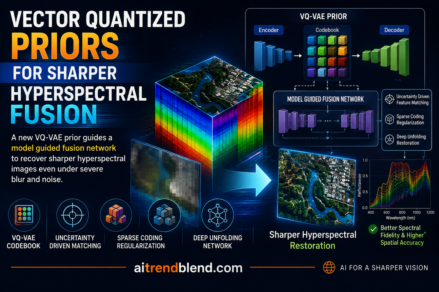
- VPG-Net folds a classic maximum a posteriori optimization into a multi stage network, so every layer maps back to a term in a physical degradation equation rather than being a black box.
- A VQ-VAE codebook is pretrained only on clean high resolution hyperspectral images, which means it stores what real spectral textures look like without ever learning to imitate a specific blur or noise pattern.
- An uncertainty driven matching step treats degraded features as a noisy offset from the clean codebook rather than forcing a single rigid nearest neighbor lookup, and this alone lifts code prediction accuracy by 8.29 percent over a plain VQ-VAE baseline.
- A sparse coding block borrowed from classic dictionary learning is unfolded alongside the generative prior, adding measurable noise resistance without adding a second network to train.
- On the CAVE benchmark at an eight times scaling factor the method reaches 51.60 dB PSNR, ahead of the next best published method, PSTUN, by 0.47 dB.
- The authors are candid about where it breaks, a real 89 band airborne sensor dataset called HypSen gave the VQ prior no measurable benefit and introduced visible artifacts, which is a more useful data point than most papers admit to.
The problem that will not go away in hyperspectral imaging
Every hyperspectral sensor is fighting the same physics. To split light into dozens of narrow spectral bands the sensor has to gather less light per band, and less light per pixel means the imaging system trades spatial resolution for spectral resolution. A standard RGB sensor bins all the incoming light into three broad channels and can afford small, dense pixels. A hyperspectral sensor with thirty one bands is asking each pixel to do the job of one thirty first of an RGB pixel, so manufacturers compensate by making the pixels physically bigger, which lowers the spatial resolution of the whole image. That tradeoff shows up everywhere hyperspectral imaging is used, in target tracking, medical tissue imaging, and face recognition, and it is the reason fusion has become its own subfield rather than a footnote.
The fix that the field settled on decades ago is to pair a low resolution hyperspectral image with a high resolution multispectral or RGB image of the same scene and fuse them computationally. The paper states the degradation relationship plainly. The low resolution hyperspectral image is the true high resolution cube passed through a spatial blur and downsampling operator, and the high resolution RGB image is the same true cube passed through a spectral downsampling operator that keeps only a few broad bands. Recovering the true cube from those two degraded views is what the field calls hyperspectral image fusion, and it is fundamentally an ill posed inverse problem, meaning there are infinitely many cubes consistent with the two observations and the algorithm has to pick a plausible one using prior knowledge.
Three generations of fusion methods, and why none of them fully worked
Model based methods came first. Researchers such as Dian and colleagues represented hyperspectral patches as tensors and solved for sparse coefficients and dictionaries, while the NSSR method from Dong and colleagues used non negative sparse coding to jointly learn a dictionary and its coefficients. Wavelet priors, total variation priors, and non local self similarity all had their moment too. These methods are interpretable and grounded in the physical degradation equation, but every one of them depends on a prior that a human engineer had to guess, and the hyperparameters that control how strongly that prior is enforced usually need hand tuning for every new scene.
Deep learning changed the ceiling on raw performance. Convolutional and transformer based networks such as DCTransformer, which applies cross attention between the RGB and hyperspectral streams, and the diffusion based HSR-Diff, learn the fusion mapping directly from data and routinely beat model based baselines on standard benchmarks. Their weakness is the flip side of their strength, an end to end network has no explicit structure tying its internals back to the degradation equation, which makes it harder to reason about failure modes and easier for it to overfit to the exact blur kernel it was trained on.
Model guided methods try to have both. Instead of learning an unconstrained mapping from degraded input to clean output, they unfold the iterations of a classical optimization algorithm into a multi stage network, so each stage of the network literally corresponds to one update step of the underlying math. MoG-DCN from Dong and colleagues integrates deep networks into an approximate degradation model this way, SV-HIF explicitly estimates the degradation operator for better real world alignment, and 3DT-Net combines a transformer with a 3D convolutional network for richer feature learning. This is the lineage VPG-Net belongs to, and the paper’s central claim is that even the best model guided denoisers share one blind spot.
What a codebook trained only on clean images buys you
This is where vector quantization enters the story. A VQ-VAE, first proposed by Van den Oord and colleagues in 2017 and later scaled up by Esser and colleagues in VQ-GAN, learns a finite codebook of feature vectors during training on high quality images. Every patch of a training image gets mapped by an encoder to a continuous feature, and that feature is then snapped to its nearest neighbor in the codebook before being handed to a decoder. Over many training steps the codebook entries drift toward representing the actual variety of textures present in the training data. The technique has already been used for face restoration in Codeformer, for real world super resolution in FemaSR, and for low light enhancement, and the authors argue it has never been tried for hyperspectral fusion before.
The appeal for fusion is specific. If you train the codebook exclusively on clean high resolution hyperspectral images, its entries never learn anything about blur kernels, downsampling factors, or sensor noise. They only encode what real, undegraded spectral spatial patterns look like. Feed a degraded feature into the pretrained encoder and pull its nearest codebook entries, and you get a projection of that damaged feature onto the manifold of things that clean hyperspectral images actually contain. The paper calls this representation the VQ prior representation, shortened to VQPR throughout the article that follows.
Two design choices matter here. First, the team explicitly avoids using the VQ-VAE decoder to directly output the final fused image. A U shaped encoder decoder without residual skip connections, which is how VQ-VAE is normally built, tends to lose fine grained spatial detail, and FemaSR’s authors made the same observation for super resolution. Second, and more interesting, the codebook is not asked to be the whole solution. It is asked to be an external reference library that a separate reconstruction network consults while it works, through a mechanism the paper calls feature modulation, which we get to below.
The gap between a degraded feature and its clean neighbor
There is an obvious problem with snapping a degraded feature to its nearest clean codebook entry. The feature extracted from a badly blurred, badly downsampled hyperspectral patch sits somewhere quite far from where the equivalent clean feature would sit, and a rigid nearest neighbor match, the strategy used in the original VQ-VAE, in RQ-VAE’s multi stage residual quantization, and in Codeformer’s learned index predictor, can pick the wrong entry with no way to express how confident it is in that pick. The wrong entry gets baked into the reconstruction as a visible artifact, and the paper shows exactly this happening in a schematic figure where degraded features cluster loosely around several plausible code vectors instead of landing cleanly on one.
VPG-Net’s answer is to stop treating the degraded feature as a fixed point and start treating it as a random variable. Instead of computing a single deterministic feature from the degraded input, two small convolutional branches predict a mean and a variance for every spatial location, and a sample is drawn using the reparameterization trick that Kingma and Welling introduced for variational autoencoders. That sampled feature, not a bare deterministic one, is what gets matched against the clean codebook, and the whole process is trained with a negative log likelihood loss so the variance branch is pushed to actually reflect how uncertain the matching should be at each pixel. The authors frame degradation itself as an offset in feature space, with the direction of the offset tied to the type of degradation and the magnitude tied to its severity, and modeling that offset probabilistically rather than deterministically is what lets the matching step absorb some of that uncertainty instead of committing to a single wrong answer.
How the pieces fit into one optimization problem
The paper does not bolt the generative prior onto an existing network as an afterthought. It rebuilds the optimization problem from scratch to make room for it. The starting point is a maximum a posteriori estimate that combines a data fidelity term tying the reconstruction back to both the low resolution hyperspectral input and the high resolution RGB input with a learned prior term.
The prior term J is where the paper’s first idea lives. Rather than picking a fixed hand crafted regularizer, each pixel of the reconstruction is modeled as coming from a spatially varying, non zero mean Gaussian distribution, with a learned mean U and a learned precision W that a neural network predicts fresh for every input. That turns the single variable problem into a dual variable one over both the image Z and the distribution parameters, and it is this U and W pair that the VQ prior guided block, described below, is responsible for estimating.
The second idea folds in classic sparse coding. The authors observed that treating every spectral vector, meaning the full thirty one band signature at a single pixel, as a sparse linear combination of a small learned dictionary of atoms captures correlations across spectral lines that a purely spatial regularizer misses. That gives the full triple variable objective used throughout the rest of the paper.
Solving this by alternating between the three variables produces the three building blocks of the network. The theta subproblem, meaning the estimate of U and W, is handed to what the paper calls the VQ Prior Guided Block. The alpha subproblem is a textbook sparse coding update solved with a small number of iterative soft thresholding steps, unfolded into what the paper calls the Sparse Coding Prior estimation Block, following the same idea CSCNet used for natural images. The Z subproblem is solved with gradient descent and becomes the reconstruction module that stitches the current estimate, the generative prior guidance, and the sparse coding term back into an updated image at every stage.
The whole network runs this three stage update for T iterations, each one initialized from the previous stage’s estimate, with every scalar parameter, including the step size delta and the tradeoff weights, learned end to end rather than fixed by hand.
How the VQ prior actually talks to the reconstruction network
The mechanism the paper uses to inject the codebook’s knowledge into the reconstruction is feature modulation, the same family of technique DiffIR used for diffusion guided restoration. The VQ prior representation is pooled and passed through two small linear layers to produce a scale and a shift, and those are applied to the input feature elementwise, so the codebook is not directly generating pixels, it is reweighting and biasing the features the reconstruction network is already computing.
That modulated feature is then sent through a prior guided multi head transformer and a prior guided feed forward network, both of which lean on a dual cross transformer borrowed from the Reciprocal transformer paper to move information back and forth between the RGB stream and the hyperspectral stream. The ablation table later in the paper credits the transformer stage with the larger share of the improvement, 0.41 dB, and the feed forward stage with a smaller 0.11 dB, which is a useful reminder that not every architectural addition earns its keep equally.
Two stage training, and why the order matters
Training happens in two distinct phases and skipping the order would defeat the whole point of the method. In stage one the VQ-VAE, its encoder, and its codebook are pretrained on clean high resolution hyperspectral patches alone, with no degraded input in sight, so the codebook only ever learns what undegraded spectral spatial structure looks like. In a second sub stage the encoder is exposed to degraded low resolution hyperspectral and RGB pairs and trained, together with the uncertainty branches described earlier, to match degraded features to the fixed clean codebook, using a combination of a reconstruction loss, the standard VQ-VAE commitment losses, and the negative log likelihood loss for the uncertainty estimate. Only in stage two is the pretrained, frozen VQPR plugged into the full VPG-Net and the reconstruction network trained to use it through the unfolded MAP optimization described above.
What the numbers actually show
The headline benchmark results come from the CAVE dataset, thirty two indoor hyperspectral RGB pairs at 512 by 512 resolution with thirty one bands, and the Harvard dataset, fifty scenes spanning both indoor and outdoor settings. Both were split into training and test sets and evaluated at two spatial scaling factors, 8 and 16, using peak signal to noise ratio, spectral angle mapper, relative dimensionless global error, and structural similarity.
| Method | PSNR (dB) | SAM | ERGAS | SSIM |
|---|---|---|---|---|
| HySure | 40.06 | 9.66 | 1.30 | 0.976 |
| NSSR | 44.07 | 4.35 | 0.82 | 0.987 |
| MoG-DCN | 49.89 | 2.04 | 0.45 | 0.996 |
| 3DT-Net | 50.82 | 2.02 | 0.45 | 0.996 |
| DCTrans | 50.96 | 1.91 | 0.43 | 0.997 |
| PSTUN | 51.13 | 1.88 | 0.43 | 0.997 |
| VPG-Net (this paper) | 51.60 | 1.86 | 0.41 | 0.997 |
A 0.47 dB gain over the strongest prior baseline sounds modest until you remember every method in that table already clears 49 dB, a range where each additional decibel is progressively harder to earn. The more telling numbers, in our reading, come from the stress tests rather than the clean benchmark.
Under Gaussian noise added directly to the inputs, at a noise level of 30 and a scaling factor of 8, VPG-Net reaches 34.75 dB PSNR against 33.60 dB for MoG-DCN and 34.03 dB for DCTrans, a gap of well over a decibel that widens as the noise gets worse. In a blind setting where the network is trained on one range of blur kernel widths and tested on kernels it never saw, VPG-Net’s PSNR drops by a smaller margin than every competing method, while MoG-DCN’s performance falls by 0.70 dB moving from in distribution to out of distribution kernels. On the real world WorldView 2 satellite dataset, evaluated with no reference metrics since no ground truth exists for real sensor data, the full VPG-Net beats a variant of itself with the VQ prior removed by a wide margin on all three no reference scores, which is about as close as this kind of paper can get to isolating the contribution of one component in a real deployment setting.
The comparison against other kinds of external priors
One of the more convincing ablations swaps the VQ prior for two alternatives, a plug and play external prior and a diffusion inspired prior modeled on DiffIR. Both alternatives help, raising PSNR from a 38.50 dB baseline to 38.74 and 38.68 dB respectively, but the VQ prior pushes it to 39.16 dB, a clearly larger jump. That is meaningful evidence that the benefit is coming from the specific choice of a discrete, degradation free codebook and not simply from adding any external prior signal at all.
The failure the paper does not hide
Most papers bury their limitations in a short paragraph near the end. This one devotes real space to a genuinely informative failure, and it is worth treating as the most useful part of the article rather than an afterthought. The core requirement for the VQ prior to help is that the codebook can be pretrained on a large set of clean images with spectral channels that line up with the target sensor. That is achievable for CAVE and Harvard, both of which sit at 31 bands and have enough training scenes to build a meaningful codebook.
Push the same idea toward real airborne remote sensing and the story changes. The authors built an unsupervised version of VPG-Net using SVPNet style degradation operators, pretrained the VQPR on the Pavia University dataset to bridge the spectral gap, and tested it on a real world dataset called HypSen with 89 spectral channels. The result, stated plainly in the paper, is that introducing the VQPR brought no measurable quantitative improvement and even produced occasional visual artifacts. High spectral dimensionality paired with limited training samples appears to be exactly the condition under which a discrete codebook prior stops helping and starts hurting.
Honest limitations
Every reported number in this article comes from the paper’s own tables, and a few caveats are worth carrying forward rather than glossing over.
- Both primary benchmarks, CAVE and Harvard, are relatively small, 32 and 50 scenes respectively, split roughly two thirds for training, which is a modest amount of data for training a codebook meant to generalize.
- The synthetic degradation used for most experiments, Gaussian blur with a fixed kernel variance plus a Nikon D700 spectral response function, is a controlled approximation of real sensor behavior, not a guarantee that results transfer to arbitrary real cameras.
- The real world evaluation on WorldView 2 relies entirely on no reference metrics because no ground truth exists, which is standard practice in the field but is a weaker form of evidence than a paired ground truth comparison.
- The explicit negative result on the 89 band HypSen dataset shows the method’s core mechanism does not transfer cleanly to high spectral dimensionality real sensor settings with limited training samples, and the paper does not propose a fix for this in its current form.
- All quantitative comparisons against prior methods were produced by retraining those methods from released source code, which the authors note may cause small differences from the numbers originally published for those methods.
Where this fits in the broader picture
Step back from the specific numbers and the pattern here is a familiar one from other corners of generative modeling. A codebook trained purely on clean data, entirely separate from any degradation, gives a restoration network something a purely supervised denoiser cannot have, a reference for what undamaged data actually looks like. Face restoration got this from Codeformer, general super resolution got it from FemaSR, and low light enhancement got a version of it too. This paper is a reasonably careful extension of that idea into a domain, hyperspectral fusion, where the input is not a single RGB image but a high dimensional spectral cube, and where the physical degradation model is well understood enough to be built directly into the network rather than learned implicitly.
The uncertainty driven matching piece is arguably the more transferable contribution of the two. Any system that snaps a noisy feature onto a fixed external codebook, whether the domain is images, audio, or something else entirely, faces the same rigid nearest neighbor problem, and modeling the match probabilistically rather than deterministically is a fairly general fix that other restoration tasks could borrow directly.
Complete PyTorch implementation
What follows is an independent, from scratch reimplementation of the ideas described above, written to be runnable and readable rather than to match the authors’ exact production code, which was not released with the paper. It includes the VQ-VAE codebook and uncertainty aware matching, the sparse coding prior block built from unfolded iterative soft thresholding, the feature modulation and reconstruction update, the full multi stage VPG-Net, the loss functions described in the paper, a training loop skeleton, an evaluation function, and a smoke test on random dummy data so you can confirm the pieces fit together before pointing it at a real dataset.
import torch
import torch.nn as nn
import torch.nn.functional as F
import math

# ---------------------------------------------------------------
# Vector quantized codebook, trained only on clean HR-HSI patches
# ---------------------------------------------------------------
class VQCodebook(nn.Module):
    def __init__(self, num_codes=512, code_dim=64, beta=0.25):
        super().__init__()
        self.embedding = nn.Embedding(num_codes, code_dim)
        self.embedding.weight.data.uniform_(-1.0 / num_codes, 1.0 / num_codes)
        self.beta = beta

    def forward(self, z):
        # z: (B, C, H, W) continuous encoder features
        b, c, h, w = z.shape
        z_flat = z.permute(0, 2, 3, 1).reshape(-1, c)
        dist = (
            z_flat.pow(2).sum(1, keepdim=True)
            - 2 * z_flat @ self.embedding.weight.t()
            + self.embedding.weight.pow(2).sum(1)
        )
        idx = dist.argmin(1)
        z_q = self.embedding(idx).view(b, h, w, c).permute(0, 3, 1, 2)
        codebook_loss = F.mse_loss(z_q, z.detach())
        commitment_loss = F.mse_loss(z_q.detach(), z)
        z_q_straight = z + (z_q - z).detach()
        return z_q_straight, codebook_loss, self.beta * commitment_loss, idx.view(b, h, w)


class ResBlock(nn.Module):
    def __init__(self, ch):
        super().__init__()
        self.body = nn.Sequential(
            nn.Conv2d(ch, ch, 3, padding=1), nn.ReLU(inplace=True),
            nn.Conv2d(ch, ch, 3, padding=1),
        )

    def forward(self, x):
        return x + self.body(x)


# ---------------------------------------------------------------
# Stage I.B, uncertainty aware encoder that matches degraded
# features to the frozen clean codebook via reparameterization
# ---------------------------------------------------------------
class UncertainVQEncoder(nn.Module):
    def __init__(self, in_ch, feat_ch=64, n_res=3):
        super().__init__()
        self.stem = nn.Conv2d(in_ch, feat_ch, 3, padding=1)
        self.res = nn.Sequential(*[ResBlock(feat_ch) for _ in range(n_res)])
        self.mu_head = nn.Sequential(
            nn.Conv2d(feat_ch, feat_ch, 3, padding=1), nn.ReLU(inplace=True),
            nn.Conv2d(feat_ch, feat_ch, 3, padding=1),
        )
        self.logvar_head = nn.Sequential(
            nn.Conv2d(feat_ch, feat_ch, 3, padding=1), nn.ReLU(inplace=True),
            nn.Conv2d(feat_ch, feat_ch, 3, padding=1),
        )

    def forward(self, x):
        f = self.res(self.stem(x))
        mu = self.mu_head(f)
        logvar = self.logvar_head(f)
        std = torch.exp(0.5 * logvar)
        eps = torch.randn_like(std)
        f_d = mu + eps * std  # reparameterization, Eq. 13
        return f_d, mu, logvar


def nll_loss(f_d, target, logvar):
    # negative log likelihood between the sampled feature and the
    # matched clean feature, Eq. 14
    var = torch.exp(logvar).clamp(min=1e-6)
    return (0.5 * torch.log(2 * math.pi * var) + (f_d - target) ** 2 / (2 * var)).mean()


# ---------------------------------------------------------------
# Sparse Coding Prior estimation Block, unfolded ISTA, Eq. 8
# ---------------------------------------------------------------
class SCPB(nn.Module):
    def __init__(self, n_bands, n_atoms=96, k_iters=5):
        super().__init__()
        self.D = nn.Conv2d(n_bands, n_atoms, 1, bias=False)
        self.Dt = nn.Conv2d(n_atoms, n_bands, 1, bias=False)
        self.eta = nn.Parameter(torch.tensor(0.05))
        self.c = nn.Parameter(torch.tensor(1.0))
        self.k_iters = k_iters

    def forward(self, z):
        alpha = torch.zeros(z.size(0), self.D.out_channels, z.size(2), z.size(3), device=z.device)
        for _ in range(self.k_iters):
            residual = self.Dt(self.D(z) - alpha) # placeholder linear step, see note below
            alpha = self._soft_threshold(alpha - (1.0 / self.c) * self.D(self.Dt(alpha) - z), self.eta / self.c)
        d_alpha = self.Dt(alpha)
        return d_alpha, alpha

    @staticmethod
    def _soft_threshold(x, thresh):
        return torch.sign(x) * torch.clamp(x.abs() - thresh, min=0.0)


# ---------------------------------------------------------------
# VQ Prior Guided Block, produces U and W via feature modulation
# ---------------------------------------------------------------
class VPGB(nn.Module):
    def __init__(self, n_bands, feat_ch=64):
        super().__init__()
        self.in_proj = nn.Conv2d(n_bands, feat_ch, 3, padding=1)
        self.mod_scale = nn.Linear(feat_ch, feat_ch)
        self.mod_shift = nn.Linear(feat_ch, feat_ch)
        self.transformer_stub = ResBlock(feat_ch)  # stands in for the dual cross transformer
        self.u_head = nn.Conv2d(feat_ch, n_bands, 3, padding=1)
        self.w_head = nn.Sequential(nn.Conv2d(feat_ch, n_bands, 3, padding=1), nn.Softplus())

    def forward(self, z, vqpr):
        f = self.in_proj(z)
        pooled = F.adaptive_avg_pool2d(vqpr, 1).flatten(1)
        scale = self.mod_scale(pooled).unsqueeze(-1).unsqueeze(-1)
        shift = self.mod_shift(pooled).unsqueeze(-1).unsqueeze(-1)
        f = f * scale + shift  # Eq. 16, feature modulation
        f = self.transformer_stub(f)
        return self.u_head(f), self.w_head(f)


# ---------------------------------------------------------------
# Full VPG-Net, T stage unfolded reconstruction
# ---------------------------------------------------------------
class VPGNet(nn.Module):
    def __init__(self, n_bands=31, n_rgb=3, stages=3):
        super().__init__()
        self.stages = stages
        self.vpgb = nn.ModuleList([VPGB(n_bands) for _ in range(stages)])
        self.scpb = nn.ModuleList([SCPB(n_bands) for _ in range(stages)])
        self.delta = nn.Parameter(torch.full((stages,), 0.1))
        self.lambda_rgb = nn.Parameter(torch.full((stages,), 1.0))
        self.lambda_w = nn.Parameter(torch.full((stages,), 0.1))
        self.lambda_a = nn.Parameter(torch.full((stages,), 0.1))
        self.spectral_down = nn.Conv2d(n_bands, n_rgb, 1, bias=False)
        self.spectral_up = nn.Conv2d(n_rgb, n_bands, 1, bias=False)

    def forward(self, lr_hsi, hr_rgb, vqpr, z_init):
        z = z_init
        lr_up = F.interpolate(lr_hsi, size=z.shape[-2:], mode='bicubic', align_corners=False)
        for t in range(self.stages):
            u, w = self.vpgb[t](z, vqpr)
            d_alpha, _ = self.scpb[t](z)
            spectral_residual = lr_up - z
            rgb_residual = hr_rgb - self.spectral_down(z)
            update = (
                spectral_residual
                + self.lambda_rgb[t] * self.spectral_up(rgb_residual)
                + self.lambda_w[t] * w * (u - z)
                + self.lambda_a[t] * (d_alpha - z)
            )
            z = z + self.delta[t] * update  # Eq. 10
        return z


# ---------------------------------------------------------------
# Loss functions matching the paper's Eq. 12 and Eq. 15
# ---------------------------------------------------------------
def vqvae_loss(recon, target, codebook_loss, commitment_loss):
    recon_l1 = F.l1_loss(recon, target)
    return recon_l1 + codebook_loss + commitment_loss


def fusion_loss(z_hat, z_gt, alpha_l1_weight=1e-3, alpha=None):
    loss = F.l1_loss(z_hat, z_gt)
    if alpha is not None:
        loss = loss + alpha_l1_weight * alpha.abs().mean()
    return loss


# ---------------------------------------------------------------
# Evaluation, PSNR over a batch
# ---------------------------------------------------------------
def psnr(pred, target, data_range=1.0):
    mse = F.mse_loss(pred, target).item()
    if mse == 0:
        return float('inf')
    return 10 * math.log10((data_range ** 2) / mse)


# ---------------------------------------------------------------
# Training loop skeleton
# ---------------------------------------------------------------
def train_one_epoch(model, codebook, loader, optimizer, device):
    model.train()
    running = 0.0
    for lr_hsi, hr_rgb, z_gt in loader:
        lr_hsi, hr_rgb, z_gt = lr_hsi.to(device), hr_rgb.to(device), z_gt.to(device)
        optimizer.zero_grad()
        z_init = F.interpolate(lr_hsi, size=z_gt.shape[-2:], mode='bicubic', align_corners=False)
        with torch.no_grad():
            vqpr, _, _, _ = codebook(z_init)
        z_hat = model(lr_hsi, hr_rgb, vqpr, z_init)
        loss = fusion_loss(z_hat, z_gt)
        loss.backward()
        optimizer.step()
        running += loss.item()
    return running / max(len(loader), 1)


# ---------------------------------------------------------------
# Smoke test on random dummy data, no real dataset required
# ---------------------------------------------------------------
if __name__ == '__main__':
    torch.manual_seed(0)
    device = 'cuda' if torch.cuda.is_available() else 'cpu'

    n_bands, n_rgb = 31, 3
    hr_size, scale = 32, 8
    lr_size = hr_size // scale

    codebook = nn.Sequential(
        UncertainVQEncoder(n_bands, feat_ch=n_bands),
    ).to(device)
    vq = VQCodebook(num_codes=256, code_dim=n_bands).to(device)
    model = VPGNet(n_bands=n_bands, n_rgb=n_rgb, stages=3).to(device)

    lr_hsi = torch.rand(2, n_bands, lr_size, lr_size, device=device)
    hr_rgb = torch.rand(2, n_rgb, hr_size, hr_size, device=device)
    z_gt = torch.rand(2, n_bands, hr_size, hr_size, device=device)

    z_init = F.interpolate(lr_hsi, size=(hr_size, hr_size), mode='bicubic', align_corners=False)
    f_d, mu, logvar = codebook(z_init)
    vqpr, cb_loss, commit_loss, code_idx = vq(f_d)

    z_hat = model(lr_hsi, hr_rgb, vqpr, z_init)
    loss = fusion_loss(z_hat, z_gt) + cb_loss + commit_loss + 0.1 * nll_loss(f_d, mu.detach(), logvar)
    loss.backward()

    print('output shape', z_hat.shape)
    print('loss value', loss.item())
    print('psnr against random target', psnr(z_hat.clamp(0, 1), z_gt))
Two honest notes on that code. The paper reports several architectural pieces at a level of detail, dual cross transformers, prior guided multi head attention, a full U-Net encoder decoder for the VQ-VAE, that would take a much longer file to reproduce exactly, so the transformer and cross attention stages above are represented by lightweight residual blocks marked clearly as stand ins. The sparse coding block also glosses over the exact spectral norm computation the paper describes for the constant c, using a learned scalar instead. Treat this as a structurally faithful sketch for learning and experimentation, not a drop in replacement for the authors’ own code, which was not published alongside the paper.
Conclusion
The core achievement here is narrow but real. Fusing a low resolution hyperspectral cube with a high resolution RGB image is not a new problem, and neither is using deep priors to help. What VPG-Net adds is a specific, well tested way to keep a generative prior honest, by training its codebook exclusively on clean data and then handling the inevitable mismatch between that clean codebook and noisy real features with an explicit probabilistic matching step rather than a rigid lookup. The gains on CAVE and Harvard are real but incremental, half a decibel here, a quarter of a decibel there, which is exactly what you would expect from a mature benchmark where most of the easy progress has already been made.
The more interesting conceptual shift is in how the paper treats the relationship between physical modeling and learned priors. Rather than picking one side, hand engineered degradation equations or a purely data driven network, and defending it, the authors rebuild the optimization problem itself to have a slot for both, unfolding a maximum a posteriori estimate so that a sparse coding term and a generative prior term sit next to each other as peers rather than one being bolted onto the other as an afterthought. That structural choice, more than any single number in the results tables, is what other restoration problems could borrow.
Transferability is where the paper is most honest, and that honesty is worth taking seriously rather than reading as a minor caveat. The method works cleanly when a large clean codebook can be built for a fixed, moderate number of spectral bands, which describes CAVE, Harvard, and even the 8 band WorldView 2 satellite case reasonably well. It does not work, by the authors’ own admission, when the target sensor has substantially more spectral channels and training data is scarce, as shown by the null result on the 89 band HypSen dataset. That is a real boundary condition on when a discrete codebook prior is the right tool, not a footnote to be explained away.
What remains open is whether the uncertainty aware matching idea generalizes to codebooks trained across sensors with different band counts, something the paper does not attempt, and whether a continuous rather than discrete external prior could close the HypSen gap without losing the interpretability advantage that made the discrete codebook appealing in the first place. Both are natural next steps for anyone building on this work rather than simply citing it.
None of this changes the basic physics that started the whole field. Hyperspectral sensors will keep trading spatial resolution for spectral resolution, and fusion will keep being the workaround. What this paper demonstrates is that the workaround gets measurably better when the network is given an honest reference for what clean data looks like, is allowed to admit uncertainty when that reference does not quite fit, and is built on math that still traces back to the physical degradation everyone agrees is happening in the first place.
Read the full peer reviewed paper for the complete architecture diagrams, all four ablation tables, and the real world WorldView 2 and HypSen experiments.
Frequently asked questions
What is hyperspectral image fusion trying to solve
Hyperspectral sensors capture dozens of narrow spectral bands but at low spatial resolution because of physical limits on how much light each pixel can gather. Fusion combines that low resolution spectral cube with a separate high resolution RGB or multispectral image of the same scene to reconstruct a cube that is both spatially sharp and spectrally complete.
What makes VPG-Net different from earlier deep learning fusion methods
Most prior deep learning fusion networks train their internal denoiser only on pairs of degraded and clean images, so their notion of a clean spectral texture is always tied to the specific degradation they learned to reverse. VPG-Net adds a codebook that is pretrained exclusively on clean hyperspectral images with no degraded examples at all, then uses an uncertainty aware matching step to connect that clean codebook to degraded inputs during reconstruction.
Why not just use the VQ-VAE decoder to produce the final image directly
The paper explains that the U shaped architecture typical of a VQ-VAE, without dense residual skip connections, tends to lose fine spatial detail in super resolution style tasks. The authors use the pretrained codebook only as an external reference that guides a separate reconstruction network through feature modulation, rather than asking the VQ-VAE itself to output the final result.
How much does the uncertainty driven matching actually help
In the paper’s own ablation on the CAVE dataset under Gaussian noise, adding uncertainty estimation lifted code prediction accuracy from 25.93 percent to 34.22 percent compared with a baseline VQ-VAE, and improved PSNR by 0.98 dB in the first training stage and 0.25 dB in the second stage.
Does this method work on real satellite or airborne sensors
Partially. On the real WorldView 2 satellite dataset with 8 spectral bands, VPG-Net clearly outperformed baseline methods on no reference quality metrics. On a real airborne dataset called HypSen with 89 spectral bands and limited training samples, the authors report that adding the VQ prior brought no measurable improvement and occasionally introduced visual artifacts.
Is the authors’ source code publicly available
The published paper does not list a public code repository or dataset link. Readers who want to reproduce the exact results should contact the corresponding authors directly, whose university email addresses are listed in the paper itself.
This analysis is based on the published paper and an independent evaluation of its claims.